Dynamic Zone Range on PDFMA [Loxx]Dynamic Zone Range on PDFMA is a Probability Density Function Moving Average oscillator with Dynamic Zones.
What is Probability Density Function?
Probability density function based MA is a sort of weighted moving average that uses probability density function to calculate the weights.
What are Dynamic Zones?
As explained in "Stocks & Commodities V15:7 (306-310): Dynamic Zones by Leo Zamansky, Ph .D., and David Stendahl"
Most indicators use a fixed zone for buy and sell signals. Here’ s a concept based on zones that are responsive to past levels of the indicator.
One approach to active investing employs the use of oscillators to exploit tradable market trends. This investing style follows a very simple form of logic: Enter the market only when an oscillator has moved far above or below traditional trading lev- els. However, these oscillator- driven systems lack the ability to evolve with the market because they use fixed buy and sell zones. Traders typically use one set of buy and sell zones for a bull market and substantially different zones for a bear market. And therein lies the problem.
Once traders begin introducing their market opinions into trading equations, by changing the zones, they negate the system’s mechanical nature. The objective is to have a system automatically define its own buy and sell zones and thereby profitably trade in any market — bull or bear. Dynamic zones offer a solution to the problem of fixed buy and sell zones for any oscillator-driven system.
An indicator’s extreme levels can be quantified using statistical methods. These extreme levels are calculated for a certain period and serve as the buy and sell zones for a trading system. The repetition of this statistical process for every value of the indicator creates values that become the dynamic zones. The zones are calculated in such a way that the probability of the indicator value rising above, or falling below, the dynamic zones is equal to a given probability input set by the trader.
To better understand dynamic zones, let's first describe them mathematically and then explain their use. The dynamic zones definition:
Find V such that:
For dynamic zone buy: P{X <= V}=P1
For dynamic zone sell: P{X >= V}=P2
where P1 and P2 are the probabilities set by the trader, X is the value of the indicator for the selected period and V represents the value of the dynamic zone.
The probability input P1 and P2 can be adjusted by the trader to encompass as much or as little data as the trader would like. The smaller the probability, the fewer data values above and below the dynamic zones. This translates into a wider range between the buy and sell zones. If a 10% probability is used for P1 and P2, only those data values that make up the top 10% and bottom 10% for an indicator are used in the construction of the zones. Of the values, 80% will fall between the two extreme levels. Because dynamic zone levels are penetrated so infrequently, when this happens, traders know that the market has truly moved into overbought or oversold territory.
Calculating the Dynamic Zones
The algorithm for the dynamic zones is a series of steps. First, decide the value of the lookback period t. Next, decide the value of the probability Pbuy for buy zone and value of the probability Psell for the sell zone.
For i=1, to the last lookback period, build the distribution f(x) of the price during the lookback period i. Then find the value Vi1 such that the probability of the price less than or equal to Vi1 during the lookback period i is equal to Pbuy. Find the value Vi2 such that the probability of the price greater or equal to Vi2 during the lookback period i is equal to Psell. The sequence of Vi1 for all periods gives the buy zone. The sequence of Vi2 for all periods gives the sell zone.
In the algorithm description, we have: Build the distribution f(x) of the price during the lookback period i. The distribution here is empirical namely, how many times a given value of x appeared during the lookback period. The problem is to find such x that the probability of a price being greater or equal to x will be equal to a probability selected by the user. Probability is the area under the distribution curve. The task is to find such value of x that the area under the distribution curve to the right of x will be equal to the probability selected by the user. That x is the dynamic zone.
Included
4 signal types
Bar coloring
Alerts
Channels fill
Buscar en scripts para "oscillator"

RSI - Dynamic Overbought/Oversold RangeDefault overbought/oversold levels of RSI does not hold good for instruments which are trending well. It happens often that instruments keep trading in single half of the range for prolonged time without even touching the other half. This also came up often in tradingview pine chat discussions where I participate regularly.
Hence, thought of creating this script to help other scriptors in finding different methods to derive dynamic high/low range of RSI. This can also be adopted for other range bound oscillators - though not inlcuded in this script.
⬜ Method
▶ Derive multitimeframe RSI. Parameters - Resolution, Source and Length are pretty straight forward. Repaint when unchecked uses previous bar value.
▶ Dynamic range detection follows below steps.
Get highest and lowest of the oscillator source for Range Length period.
Use Detection method further to refine the highest and lowest range. If detection method is "highlow", then it looks for lowest value for high range and highest value for low range. If not, uses moving average.
◽Note: Detection range length is used only for finding highest and lowest of Oscillator value ranges. Further detection range method of highlow and other moving average types use Oscillator length.

Smoke And MirrorsSmoke And Mirrors is an indicator combining few simple but often used indicators to a delightfully visual presentation. Smoke And Mirrors features a generic SMA from where it derives BBands and a Standard Deviation band, and in it's default configuration offers a small timescale Average True Range and also matches the generic SMA against VWAP in an oscillatory fashion. And that's not all! It also has very unique voodoo on top of it all, charting the distance between open and close and the distance between high and low based on the average of open, close, high and low. It's pretty intuitive and while the settings have numerous variables to tweak, they're mostly related to how the colors are displayed so you can set it up to match your current charts colors. The default settings are meant for charts with a normal change of around 1 unit, so if you're charting something that's in it's tens of thousands and varies daily by a 1000 or more, you might want to tone the "rate-of-change" numbers down to all the way to 1. Other than that, it's recommended that you play around with the numbers a little bit so that you know which band represents which indicator.
Don't hesitate to use any or all parts of the indicator in your own scripts! There's a handy hsva function that yields rgb color with transparency based on hue(0-360), saturation (0-1), value (0-1) and alpha (0-1) and plenty of examples on how to utilize it.

MarketVision BWith Special Thanks to Everyone who has gone before me, and who have both allowed me given me permission to bring my version of Market Cipher to the World
Especially LazyBear for his amazing Wave Trend Oscillator and for Aevir, falconCoin, vumanchu, Crypto_Spike and others who have freely brought MarketCipher to the Tradingview Community
Also special mention to RicardoSantos for his Divergence script
MarketVision B - My take on MarketCipher B / Market Cipher B, Ive just put outlines on the Wave Trend to add to the Visual Appeal and Added a Trend Meter and a few more options for the Oscillators
Nice To Look At
Oscillator 1 Choose Between - RSI, MFI and Ultimate Oscillator
For Stochastics Choose Between Standard and RSI Stochastics and for the source you can choose On Balance Volume
Wave Trend
Money Flow
Trend Meter & Signals Bar
Divergences are marked, However they are easy to spot and it is better to train your eyes to spot them before the indicator marks them out
Lots of Alerts and Loads of ways to trade using MarketVision
PS: You can make this look like the original by adjusting the parameters in the menu

Stochastic On Balance Volume(not sure why the text in the image above is messed up; it looked good before publishing. The oscillators above are (from top to bottom) StochOBV, OBVOSC (LazyBear), OBV)
Applies the Stochastic Oscillator to OBV the same way StochRSI applies the Stochastic Oscillator to RSI.
Features:
- Bounded between 0 and 100, so it may be used for overbought/oversold alerts;
- Uses two lines for crossing signals similar to Stoch and StochRSI;
- Only considers recent OBV action, similar to how StochRSI only considers recent RSI action;
It can be used for simple signals, divergence, trend lines, and any other method you'd use StochRSI for.
The OBV calculation is from LazyBear's OBVOSC script here , so thank you for your script.

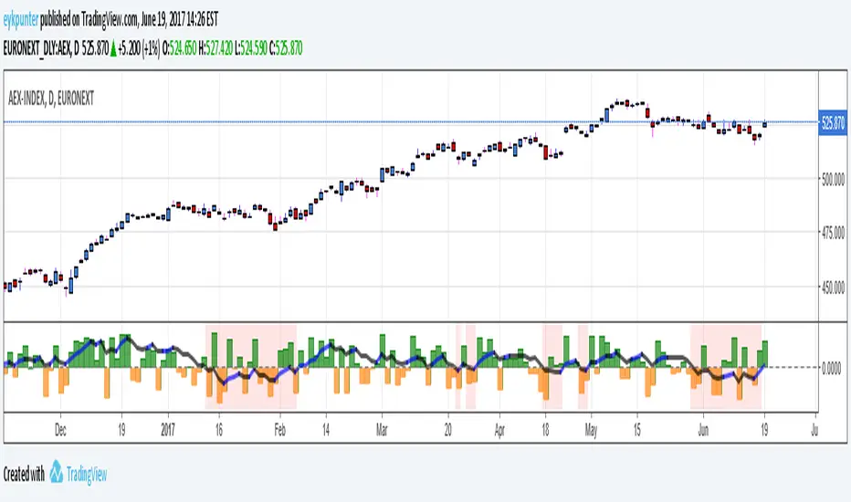
True Balance of powerThis is an improvement of the script published by LazyBear,
The improvements are:
1. it includes gaps because it uses true range in stead of the current bar,
2. it has been turned into a percent oscillator as the basic algorithm belongs in the family of stochastic oscillators.
Unlike the usual stochatics I refrained from over the top averaging and smoothing, nor did I attempt a signal line. There’s no need to make a mock MACD.
The indicator should be interpreted as a stochastics, the difference between Stochs and MACD is that stochs report inclinations, i.e. in which direction the market is edging, while MACD reports movements, in which direction the market is moving. Stochs are an early indicator, MACD is lagging. The emoline is a 30 period linear regression, I use linear regressions because these have no lagging, react immidiately to changes, I use a 30 period version because that is not so nervous. You might say that an MA gives an average while a linear regression gives an ‘over all’ of the periods.
The back ground color is red when the emoline is below zero, that is where the market ‘looks down’, white where the market ‘looks up’. This doesn’t mean that the market will actually go down or up, it may allways change its mind.
Have fun and take care, Eykpunter.
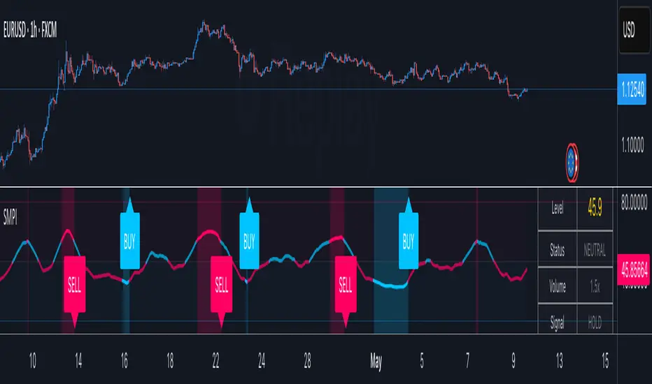
Smart Money Proxy IndexOverview
The Smart Money Proxy Index (SMPI) is an educational tool that attempts to identify potential institutional-style behavior patterns using publicly available market data. This comprehensive tool combines multiple institutional analysis techniques into a single, easy-to-read 0-100 oscillator.
Important Disclaimer
This is an educational proxy indicator that analyzes volume and price patterns. It cannot identify actual institutional trading activity and should not be interpreted as tracking real "smart money." Use for educational purposes and combine with other analysis methods.
Inspiration & Methodology
This indicator is inspired by MAPsignals' Big Money Index (BMI) methodology but uses publicly available price and volume data with original calculations. This is an independent educational interpretation designed to teach smart money concepts to retail traders.
What It Analyzes
SMPI tracks potential "smart money" activity by combining:
Block Trading Detection - Identifies unusual volume surges with significant price impact
Money Flow Analysis - Volume-weighted price pressure using Money Flow Index
Accumulation/Distribution Patterns - Modified On-Balance Volume signals
Institutional Control Proxy - End-of-day positioning and control analysis
Key Features
– Multi-Component Analysis - Combines 4 different institutional detection methods
– BMI-Style 0-100 Scale - Familiar oscillator range with clear extreme levels
– Professional Visualization - Dynamic colors, gradient fills, and clean data table
– Comprehensive Alerts - Buy/sell signals plus divergence detection
– Fully Customizable - Adjust all parameters, colors, and display options
– Non-Repainting Signals - All alerts use confirmed data for reliability
– Educational Focus - Designed to teach institutional flow concepts
How to Interpret
Above 80: Potential smart money distribution phase (bearish pressure)
Below 20: Potential smart money accumulation phase (bullish opportunity)
Signal Generation: Buy signals when crossing above 20, sell signals when crossing below 80
Divergences: Price vs SMPI divergences can signal potential trend changes
Volume Confirmation: Higher volume ratios strengthen signal reliability
Best Practices
Timeframes: Works best on higher timeframes for institutional behavior analysis
Confirmation: Combine with other technical analysis tools and market context
Volume: Pay attention to volume confirmation in the data table
Context: Consider overall market conditions and fundamental factors
Risk Management: Not recommended as standalone trading system
Customizable Parameters
Block Volume Threshold: Sensitivity for unusual volume detection (default: 2.5x average)
SMPI Smoothing Period: Index calculation smoothing (default: 25 bars)
Extreme Levels: Overbought/oversold thresholds (default: 80/20)
Money Flow Length: MFI calculation period (default: 14)
Visual Options: Colors, signals, and display preferences
Available Alerts
Buy Signal: SMPI crosses above oversold level (20)
Sell Signal: SMPI crosses below overbought level (80)
Extreme Levels: Alerts when reaching overbought/oversold zones
Divergence Detection: Bullish and bearish price vs SMPI divergences
Educational Purpose & Limitations
This indicator is designed as an educational proxy for understanding institutional flow concepts. It analyzes publicly available price and volume data to identify potential smart money behavior patterns.
Cannot access actual institutional transaction data
Signals may be slower than day-trading indicators (intentionally designed for institutional timeframes)
Should be used in conjunction with other analysis methods
Past performance does not guarantee future results
What Makes This Different
Unlike simple volume or momentum indicators, SMPI combines multiple institutional analysis techniques into one comprehensive tool. The multi-component approach provides a more robust view of potential smart money activity.
StochFusion – Multi D-LineStochFusion – Multi D-Line
An advanced fusion of four Stochastic %D lines into one powerful oscillator.
What it does:
Combines four user-weighted Stochastic %D lines—from fastest (9,3) to slowest (60,10)—into a single “Fusion” line that captures both short-term and long-term momentum in one view.
How to use:
Adjust the four weights (0–10) to emphasize the speed of each %D component.
Watch the Fusion line crossing key zones:
– Above 80 → overbought condition, potential short entry.
– Below 20 → oversold condition, potential long entry.
– Around 50 → neutral/midline, watch for trend shifts.
Applications:
Entry/exit filter: Only take trades when the Fusion line confirms zone exits.
Trend confirmation: Analyze slope and cross of the midline for momentum strength.
Multi-timeframe alignment: Use on different chart resolutions to find confluence.
Tips & Tricks:
Default weights give more influence to slower %D—good for trend-focused strategies.
Equal weights provide a balanced oscillator that mimics an ensemble average.
Experiment: Increase the fastest weight to capture early reversal signals.
Developed by: TradeQUO — inspired by DayTraderRadio John
“The best momentum indicator is the one you adapt to your own trading rhythm.”

Reflexivity Resonance Factor (RRF) - Quantum Flow Reflexivity Resonance Factor (RRF) – Quantum Flow
See the Feedback Loops. Anticipate the Regime Shift.
What is the RRF – Quantum Flow?
The Reflexivity Resonance Factor (RRF) – Quantum Flow is a next-generation market regime detector and energy oscillator, inspired by George Soros’ theory of reflexivity and modern complexity science. It is designed for traders who want to visualize the hidden feedback loops between market perception and participation, and to anticipate explosive regime shifts before they unfold.
Unlike traditional oscillators, RRF does not just measure price momentum or volatility. Instead, it models the dynamic feedback between how the market perceives itself (perception) and how it acts on that perception (participation). When these feedback loops synchronize, they create “resonance” – a state of amplified reflexivity that often precedes major market moves.
Theoretical Foundation
Reflexivity: Markets are not just driven by external information, but by participants’ perceptions and their actions, which in turn influence future perceptions. This feedback loop can create self-reinforcing trends or sudden reversals.
Resonance: When perception and participation align and reinforce each other, the market enters a high-energy, reflexive state. These “resonance” events often mark the start of new trends or the climax of existing ones.
Energy Field: The indicator quantifies the “energy” of the market’s reflexivity, allowing you to see when the crowd is about to act in unison.
How RRF – Quantum Flow Works
Perception Proxy: Measures the rate of change in price (ROC) over a configurable period, then smooths it with an EMA. This models how quickly the market’s collective perception is shifting.
Participation Proxy: Uses a fast/slow ATR ratio to gauge the intensity of market participation (volatility expansion/contraction).
Reflexivity Core: Multiplies perception and participation to model the feedback loop.
Resonance Detection: Applies Z-score normalization to the absolute value of reflexivity, highlighting when current feedback is unusually strong compared to recent history.
Energy Calculation: Scales resonance to a 0–100 “energy” value, visualized as a dynamic background.
Regime Strength: Tracks the percentage of bars in a lookback window where resonance exceeded the threshold, quantifying the persistence of reflexive regimes.
Inputs:
🧬 Core Parameters
Perception Period (pp_roc_len, default 14): Lookback for price ROC.
Lower (5–10): More sensitive, for scalping (1–5min).
Default (14): Balanced, for 15min–1hr.
Higher (20–30): Smoother, for 4hr–daily.
Perception Smooth (pp_smooth_len, default 7): EMA smoothing for perception.
Lower (3–5): Faster, more detail.
Default (7): Balanced.
Higher (10–15): Smoother, less noise.
Participation Fast (prp_fast_len, default 7): Fast ATR for immediate volatility.
5–7: Scalping.
7–10: Day trading.
10–14: Swing trading.
Participation Slow (prp_slow_len, default 21): Slow ATR for baseline volatility.
Should be 2–4x fast ATR.
Default (21): Works with fast=7.
⚡ Signal Configuration
Resonance Window (res_z_window, default 50): Z-score lookback for resonance normalization.
20–30: More reactive.
50: Medium-term.
100+: Very stable.
Primary Threshold (rrf_threshold, default 1.5): Z-score level for “Active” resonance.
1.0–1.5: More signals.
1.5: Balanced.
2.0+: Only strong signals.
Extreme Threshold (rrf_extreme, default 2.5): Z-score for “Extreme” resonance.
2.5: Major regime shifts.
3.0+: Only the most extreme.
Regime Window (regime_window, default 100): Lookback for regime strength (% of bars with resonance spikes).
Higher: More context, slower.
Lower: Adapts quickly.
🎨 Visual Settings
Show Resonance Flow (show_flow, default true): Plots the main resonance line with glow effects.
Show Signal Particles (show_particles, default true): Circular markers at active/extreme resonance points.
Show Energy Field (show_energy, default true): Background color based on resonance energy.
Show Info Dashboard (show_dashboard, default true): Status panel with resonance metrics.
Show Trading Guide (show_guide, default true): On-chart quick reference for interpreting signals.
Color Mode (color_mode, default "Spectrum"): Visual theme for all elements.
“Spectrum”: Cyan→Magenta (high contrast)
“Heat”: Yellow→Red (heat map)
“Ocean”: Blue gradients (easy on eyes)
“Plasma”: Orange→Purple (vibrant)
Color Schemes
Dynamic color gradients are used for all plots and backgrounds, adapting to both resonance intensity and direction:
Spectrum: Cyan/Magenta for bullish/bearish resonance.
Heat: Yellow/Red for bullish, Blue/Purple for bearish.
Ocean: Blue gradients for both directions.
Plasma: Orange/Purple for high-energy states.
Glow and aura effects: The resonance line is layered with multiple glows for depth and signal strength.
Background energy field: Darker = higher energy = stronger reflexivity.
Visual Logic
Main Resonance Line: Shows the smoothed resonance value, color-coded by direction and intensity.
Glow/Aura: Multiple layers for visual depth and to highlight strong signals.
Threshold Zones: Dotted lines and filled areas mark “Active” and “Extreme” resonance zones.
Signal Particles: Circular markers at each “Active” (primary threshold) and “Extreme” (extreme threshold) event.
Dashboard: Top-right panel shows current status (Dormant, Building, Active, Extreme), resonance value, energy %, and regime strength.
Trading Guide: Bottom-right panel explains all states and how to interpret them.
How to Use RRF – Quantum Flow
Dormant (💤): Market is in equilibrium. Wait for resonance to build.
Building (🌊): Resonance is rising but below threshold. Prepare for a move.
Active (🔥): Resonance exceeds primary threshold. Reflexivity is significant—consider entries or exits.
Extreme (⚡): Resonance exceeds extreme threshold. Major regime shift likely—watch for trend acceleration or reversal.
Energy >70%: High conviction, crowd is acting in unison.
Above 0: Bullish reflexivity (positive feedback).
Below 0: Bearish reflexivity (negative feedback).
Regime Strength: % of bars in “Active” state—higher = more persistent regime.
Tips:
- Use lower lookbacks for scalping, higher for swing trading.
- Combine with price action or your own system for confirmation.
- Works on all assets and timeframes—tune to your style.
Alerts
RRF Activation: Resonance crosses above primary threshold.
RRF Extreme: Resonance crosses above extreme threshold.
RRF Deactivation: Resonance falls below primary threshold.
Originality & Usefulness
RRF – Quantum Flow is not a mashup of existing indicators. It is a novel oscillator that models the feedback loop between perception and participation, then quantifies and visualizes the resulting resonance. The multi-layered color logic, energy field, and regime strength dashboard are unique to this script. It is designed for anticipation, not confirmation—helping you see regime shifts before they are obvious in price.
Chart Info
Script Name: Reflexivity Resonance Factor (RRF) – Quantum Flow
Recommended Use: Any asset, any timeframe. Tune parameters to your style.
Disclaimer
This script is for research and educational purposes only. It does not provide financial advice or direct buy/sell signals. Always use proper risk management and combine with your own strategy. Past performance is not indicative of future results.
Trade with insight. Trade with anticipation.
— Dskyz , for DAFE Trading Systems

Stochastic Fusion Elite [trade_lexx]📈 Stochastic Fusion Elite is your reliable trading assistant!
📊 What is Stochastic Fusion Elite ?
Stochastic Fusion Elite is a trading indicator based on a stochastic oscillator. It analyzes the rate of price change and generates buy or sell signals based on various technical analysis methods.
💡 The main components of the indicator
📊 Stochastic oscillator (K and D)
Stochastic shows the position of the current price relative to the price range for a certain period. Values above 80 indicate overbought (an early sale is possible), and values below 20 indicate oversold (an early purchase is possible).
📈 Moving Averages (MA)
The indicator uses 10 different types of moving averages to smooth stochastic lines.:
- SMA: Simple moving average
- EMA: Exponential moving average
- WMA: Weighted moving average
- HMA: Moving Average Scale
- KAMA: Kaufman Adaptive Moving Average
- VWMA: Volume-weighted moving average
- ALMA: Arnaud Legoux Moving Average
- TEMA: Triple exponential moving average
- ZLEMA: zero delay exponential moving average
- DEMA: Double exponential moving average
The choice of the type of moving average affects the speed of the indicator's response to market changes.
🎯 Bollinger Bands (BB)
Bands around the moving average that widen and narrow depending on volatility. They help determine when the stochastic is out of the normal range.
🔄 Divergences
Divergences show discrepancies between price and stochastic:
- Bullish divergence: price is falling and stochastic is rising — an upward reversal is possible
- Bearish divergence: the price is rising, and stochastic is falling — a downward reversal is possible
🔍 Indicator signals
1️⃣ KD signals (K and D stochastic lines)
- Buy signal:
- What happens: the %K line crosses the %D line from bottom to top
- What does it look like: a green triangle with the label "KD" under the chart and the label "Buy" below the bar
- What does this mean: the price is gaining an upward momentum, growth is possible
- Sell signal:
- What happens: the %K line crosses the %D line from top to bottom
- What it looks like: a red triangle with the label "KD" above the chart and the label "Sell" above the bar
- What does this mean: the price is losing its upward momentum, possibly falling
2️⃣ Moving Average Signals (MA)
- Buy Signal:
- What happens: stochastic crosses the moving average from bottom to top
- What it looks like: a green triangle with the label "MA" under the chart and the label "Buy" below the bar
- What does this mean: stochastic is starting to accelerate upward, price growth is possible
- Sell signal:
- What happens: stochastic crosses the moving average from top to bottom
- What it looks like: a red triangle with the label "MA" above the chart and the label "Sell" above the bar
- What does this mean: stochastic is starting to accelerate downwards, a price drop is possible
3️⃣ Bollinger Band Signals (BB)
- Buy signal:
- What happens: stochastic crosses the lower Bollinger band from bottom to top
- What it looks like: a green triangle with the label "BB" under the chart and the label "Buy" below the bar
- What does this mean: stochastic was too low and is now starting to recover
- Sell signal:
- What happens: Stochastic crosses the upper Bollinger band from top to bottom
- What it looks like: a red triangle with a "BB" label above the chart and a "Sell" label above the bar
- What does this mean: stochastic was too high and is now starting to decline
4️⃣ Divergence Signals (Div)
- Buy Signal (Bullish Divergence):
- What's happening: the price is falling, and stochastic is forming higher lows
- What it looks like: a green triangle with a "Div" label under the chart and a "Buy" label below the bar
- What does this mean: despite the falling price, the momentum is already changing in an upward direction
- Sell signal (bearish divergence):
- What's going on: the price is rising, and stochastic is forming lower highs
- What it looks like: a red triangle with a "Div" label above the chart and a "Sell" label above the bar
- What does this mean: despite the price increase, the momentum is already weakening
🛠️ Filters to filter out false signals
1️⃣ Minimum distance between the signals
- What it does: sets the minimum number of candles between signals
- Why it is needed: prevents signals from being too frequent during strong market fluctuations
- How to set it up: Set the number from 0 and above (default: 5)
2️⃣ "Waiting for the opposite signal" mode
- What it does: waits for a signal in the opposite direction before generating a new signal
- Why you need it: it helps you not to miss important trend reversals
- How to set up: just turn the function on or off
3️⃣ Filter by stochastic levels
- What it does: generates signals only when the stochastic is in the specified ranges
- Why it is needed: it helps to catch the moments when the market is oversold or overbought
- How to set up:
- For buy signals: set a range for oversold (for example, 1-20)
- For sell signals: set a range for overbought (for example, 80-100)
4️⃣ MFI filter
- What it does: additionally checks the values of the cash flow index (MFI)
- Why it is needed: confirms stochastic signals with cash flow data
- How to set it up:
- For buy signals: set the range for oversold MFI (for example, 1-25)
- For sell signals: set the range for overbought MFI (for example, 75-100)
5️⃣ The RSI filter
- What it does: additionally checks the RSI values to confirm the signals
- Why it is needed: adds additional confirmation from another popular indicator
- How to set up:
- For buy signals: set the range for oversold MFI (for example, 1-30)
- For sell signals: set the range for overbought MFI (for example, 70-100)
🔄 Signal combination modes
1️⃣ Normal mode
- How it works: all signals (KD, MA, BB, Div) work independently of each other
- When to use it: for general market analysis or when learning how to work with the indicator
2️⃣ "AND" Mode ("AND Mode")
- How it works: the alarm appears only when several conditions are triggered simultaneously
- Combination options:
- KD+MA: signals from the KD and moving average lines
- KD+BB: signals from KD lines and Bollinger bands
- KD+Div: signals from the KD and divergence lines
- KD+MA+BB: three signals simultaneously
- KD+MA+Div: three signals at the same time
- KD+BB+Div: three signals at the same time
- KD+MA+BB+Div: all four signals at the same time
- When to use: for more reliable but rare signals
🔌 Connecting to trading strategies
The indicator can be connected to your trading strategies using 6 different channels.:
1. Connector KD signals: connects only the signals from the intersection of lines K and D
2. Connector MA signals: connects only signals from moving averages
3. Connector BB signal: connects only the signals from the Bollinger bands
4. Connector divergence signals: connects only divergence signals
5. Combined Connector: connects any signals
6. Connector for "And" mode: connects only combined signals
🔔 Setting up alerts
The indicator can send alerts when alarms appear.:
- Alerts for KD: when the %K line crosses the %D line
- Alerts for MA: when stochastic crosses the moving average
- Alerts for BB: when stochastic crosses the Bollinger bands
- Divergence alerts: when a divergence is detected
- Combined alerts: for all types of alarms
- Alerts for "And" mode: for combined signals
🎭 What does the indicator look like on the chart ?
- Main lines K and D: blue and orange lines
- Overbought/oversold levels: horizontal lines at levels 20 and 80
- Middle line: dotted line at level 50
- Stochastic Moving Average: yellow line
- Bollinger bands: green lines around the moving average
- Signals: green and red triangles with corresponding labels
📚 How to start using Stochastic Fusion Elite
1️⃣ Initial setup
- Add an indicator to your chart
- Select the types of signals you want to use (KD, MA, BB, Div)
- Adjust the period and smoothing for the K and D lines
2️⃣ Filter settings
- Set the distance between the signals to get rid of unnecessary noise
- Adjust stochastic, MFI and RSI levels depending on the volatility of your asset
- If you need more reliable signals, turn on the "Waiting for the opposite signal" mode.
3️⃣ Operation mode selection
- First, use the standard mode to see all possible signals.
- When you get comfortable, try the "And" mode for rarer signals.
4️⃣ Setting up Alerts
- Select the types of signals you want to be notified about
- Set up alerts for these types of signals
5️⃣ Verification and adaptation
- Check the operation of the indicator on historical data
- Adjust the parameters for a specific asset
- Adapt the settings to your trading style
🌟 Usage examples
For trend trading
- Use the KD and MA signals in the direction of the main trend
- Set the distance between the signals
- Set stricter levels for filters
For trading in a sideways range
- Use BB signals to detect bounces from the range boundaries
- Use a stochastic level filter to confirm overbought/oversold conditions
- Adjust the Bollinger bands according to the width of the range
To determine the pivot points
- Pay attention to the divergence signals
- Set the distance between the signals
- Check the MFI and RSI filters for additional confirmation

Machine Learning Momentum Index (MLMI) [Zeiierman]█ Overview
The Machine Learning Momentum Index (MLMI) represents the next step in oscillator trading. By blending traditional momentum analysis with machine learning, MLMI delivers a potent and dynamic tool that aligns with the complexities of modern financial landscapes. Offering traders an adaptive way to understand and act on market momentum and trends, this oscillator provides real-time insights into market momentum and prevailing trends.
█ How It Works:
Momentum Analysis: MLMI employs a dual-layer analysis, utilizing quick and slow weighted moving averages (WMA) of the Relative Strength Index (RSI) to gauge the market's momentum and direction.
Machine Learning Integration: Through the k-Nearest Neighbors (k-NN) algorithm, MLMI intelligently examines historical data to make more accurate momentum predictions, adapting to the intricate patterns of the market.
MLMI's precise calculation involves:
Weighted Moving Averages: Calculations of quick (5-period) and slow (20-period) WMAs of the RSI to track short-term and long-term momentum.
k-Nearest Neighbors Algorithm: Distances between current parameters and previous data are measured, and the nearest neighbors are used for predictive modeling.
Trend Analysis: Recognition of prevailing trends through the relationship between quick and slow-moving averages.
█ How to use
The Machine Learning Momentum Index (MLMI) can be utilized in much the same way as traditional trend and momentum oscillators, providing key insights into market direction and strength. What sets MLMI apart is its integration of artificial intelligence, allowing it to adapt dynamically to market changes and offer a more nuanced and responsive analysis.
Identifying Trend Direction and Strength: The MLMI serves as a tool to recognize market trends, signaling whether the momentum is upward or downward. It also provides insights into the intensity of the momentum, helping traders understand both the direction and strength of prevailing market trends.
Identifying Consolidation Areas: When the MLMI Prediction line and the WMA of the MLMI Prediction line become flat/oscillate around the mid-level, it's a strong sign that the market is in a consolidation phase. This insight from the MLMI allows traders to recognize periods of market indecision.
Recognizing Overbought or Oversold Conditions: By identifying levels where the market may be overbought or oversold, MLMI offers insights into potential price corrections or reversals.
█ Settings
Prediction Data (k)
This parameter controls the number of neighbors to consider while making a prediction using the k-Nearest Neighbors (k-NN) algorithm. By modifying the value of k, you can change how sensitive the prediction is to local fluctuations in the data.
A smaller value of k will make the prediction more sensitive to local variations and can lead to a more erratic prediction line.
A larger value of k will consider more neighbors, thus making the prediction more stable but potentially less responsive to sudden changes.
Trend length
This parameter controls the length of the trend used in computing the momentum. This length refers to the number of periods over which the momentum is calculated, affecting how quickly the indicator reacts to changes in the underlying price movements.
A shorter trend length (smaller momentumWindow) will make the indicator more responsive to short-term price changes, potentially generating more signals but at the risk of more false alarms.
A longer trend length (larger momentumWindow) will make the indicator smoother and less responsive to short-term noise, but it may lag in reacting to significant price changes.
Please note that the Machine Learning Momentum Index (MLMI) might not be effective on higher timeframes, such as daily or above. This limitation arises because there may not be enough data at these timeframes to provide accurate momentum and trend analysis. To overcome this challenge and make the most of what MLMI has to offer, it's recommended to use the indicator on lower timeframes.
-----------------
Disclaimer
The information contained in my Scripts/Indicators/Ideas/Algos/Systems does not constitute financial advice or a solicitation to buy or sell any securities of any type. I will not accept liability for any loss or damage, including without limitation any loss of profit, which may arise directly or indirectly from the use of or reliance on such information.
All investments involve risk, and the past performance of a security, industry, sector, market, financial product, trading strategy, backtest, or individual's trading does not guarantee future results or returns. Investors are fully responsible for any investment decisions they make. Such decisions should be based solely on an evaluation of their financial circumstances, investment objectives, risk tolerance, and liquidity needs.
My Scripts/Indicators/Ideas/Algos/Systems are only for educational purposes!

(mab) Volume IndexThis script implements the (mab) Volume Index (MVI) which is a volume momentum oscillator. The formula is similar to the formula of RSI but uses volume instead of price. The price is calculated as the average of open, high, low and close prices and is used to determine if the volume is counted as up-volume or down-volume.
I created MVI to replace OBV on my charts, because OBV is not as simple to read and find e.g. divergences. MVI is much easier to read because it is an oscillator with a minimum value of 0 and a maximum value of 100. It's easy to find divergences too. I like to display MVI over the volume bars. However, you can display it in a separate pain as well.
[blackcat] L3 Gann SlopeLevel 3
Background
William Gann (Wilian D. Gann) is one of the most famous investors in the twentieth century. His outstanding achievements in the stock and futures markets are unparalleled. The theory he created that perfectly combines time and price has been It is still talked about and highly praised by the investment community.
Function
The slope is the degree of the angle line relative to the time axis (X axis). Volatility is the ratio of unit amplitude to unit time. At the heart of Gann angles is the determination of volatility. Gann angle is the movement of price defined by time unit and price unit. Each angle is determined by the relationship between time and price. In the rising angle, the angle with the larger slope means that the stock price is rising stronger and falling. In a trend line, the larger the slope, the stronger the downtrend.
This technical indicator speaks of the Gann slope expressed as an oscillator. Its value varies from 0 to 100. The positive slope means rising, and the negative slope means falling. For rising and falling, the strength of rising and falling is distinguished by the thickness and color of the oscillating line:
1. The thin white line represents the basic oscillator curve and has no special meaning.
2. Light red indicates that an uptrend is established, and dark red indicates a very strong uptrend.
3. Light green indicates an established downtrend, dark green indicates a very strong downtrend.
Remarks
Feedbacks are appreciated.
DMI Stochastic Momentum IndexConcepts
This is an improved version of the "DMI Stochastic Extreme Refurbished" indicator.
For more information on the main concepts of this indicator, please access this link:
The difference is that here, instead of using the traditional stochastic oscillator, I implemented the use of the Stochastic Momentum Index (SMI).
Stochastic Momentum Index (SMI)
The SMI is considered a refinement of the stochastic oscillator.
It calculates the distance of the current closing price as it relates to the median of the high/low range of price.
William Blau developed the SMI, which attempts to provide a more reliable indicator, less subject to false swings.
The original stochastic is limited to values from 0 to 100, while the SMI varies between the range of -100 to 100.
(Investopedia)
It is worth mentioning that the SMI presented in this script applies to the DMI value, not the screen price.

Softmax Normalized T3 Histogram [Loxx]Softmax Normalized T3 Histogram is a T3 moving average that is morphed into a normalized oscillator from -1 to 1.
What is the Softmax function?
The softmax function, also known as softargmax: or normalized exponential function, converts a vector of K real numbers into a probability distribution of K possible outcomes. It is a generalization of the logistic function to multiple dimensions, and used in multinomial logistic regression. The softmax function is often used as the last activation function of a neural network to normalize the output of a network to a probability distribution over predicted output classes, based on Luce's choice axiom.
What is the T3 moving average?
Better Moving Averages Tim Tillson
November 1, 1998
Tim Tillson is a software project manager at Hewlett-Packard, with degrees in Mathematics and Computer Science. He has privately traded options and equities for 15 years.
Introduction
"Digital filtering includes the process of smoothing, predicting, differentiating, integrating, separation of signals, and removal of noise from a signal. Thus many people who do such things are actually using digital filters without realizing that they are; being unacquainted with the theory, they neither understand what they have done nor the possibilities of what they might have done."
This quote from R. W. Hamming applies to the vast majority of indicators in technical analysis . Moving averages, be they simple, weighted, or exponential, are lowpass filters; low frequency components in the signal pass through with little attenuation, while high frequencies are severely reduced.
"Oscillator" type indicators (such as MACD , Momentum, Relative Strength Index ) are another type of digital filter called a differentiator.
Tushar Chande has observed that many popular oscillators are highly correlated, which is sensible because they are trying to measure the rate of change of the underlying time series, i.e., are trying to be the first and second derivatives we all learned about in Calculus.
We use moving averages (lowpass filters) in technical analysis to remove the random noise from a time series, to discern the underlying trend or to determine prices at which we will take action. A perfect moving average would have two attributes:
It would be smooth, not sensitive to random noise in the underlying time series. Another way of saying this is that its derivative would not spuriously alternate between positive and negative values.
It would not lag behind the time series it is computed from. Lag, of course, produces late buy or sell signals that kill profits.
The only way one can compute a perfect moving average is to have knowledge of the future, and if we had that, we would buy one lottery ticket a week rather than trade!
Having said this, we can still improve on the conventional simple, weighted, or exponential moving averages. Here's how:
Two Interesting Moving Averages
We will examine two benchmark moving averages based on Linear Regression analysis.
In both cases, a Linear Regression line of length n is fitted to price data.
I call the first moving average ILRS, which stands for Integral of Linear Regression Slope. One simply integrates the slope of a linear regression line as it is successively fitted in a moving window of length n across the data, with the constant of integration being a simple moving average of the first n points. Put another way, the derivative of ILRS is the linear regression slope. Note that ILRS is not the same as a SMA ( simple moving average ) of length n, which is actually the midpoint of the linear regression line as it moves across the data.
We can measure the lag of moving averages with respect to a linear trend by computing how they behave when the input is a line with unit slope. Both SMA (n) and ILRS(n) have lag of n/2, but ILRS is much smoother than SMA .
Our second benchmark moving average is well known, called EPMA or End Point Moving Average. It is the endpoint of the linear regression line of length n as it is fitted across the data. EPMA hugs the data more closely than a simple or exponential moving average of the same length. The price we pay for this is that it is much noisier (less smooth) than ILRS, and it also has the annoying property that it overshoots the data when linear trends are present.
However, EPMA has a lag of 0 with respect to linear input! This makes sense because a linear regression line will fit linear input perfectly, and the endpoint of the LR line will be on the input line.
These two moving averages frame the tradeoffs that we are facing. On one extreme we have ILRS, which is very smooth and has considerable phase lag. EPMA has 0 phase lag, but is too noisy and overshoots. We would like to construct a better moving average which is as smooth as ILRS, but runs closer to where EPMA lies, without the overshoot.
A easy way to attempt this is to split the difference, i.e. use (ILRS(n)+EPMA(n))/2. This will give us a moving average (call it IE /2) which runs in between the two, has phase lag of n/4 but still inherits considerable noise from EPMA. IE /2 is inspirational, however. Can we build something that is comparable, but smoother? Figure 1 shows ILRS, EPMA, and IE /2.
Filter Techniques
Any thoughtful student of filter theory (or resolute experimenter) will have noticed that you can improve the smoothness of a filter by running it through itself multiple times, at the cost of increasing phase lag.
There is a complementary technique (called twicing by J.W. Tukey) which can be used to improve phase lag. If L stands for the operation of running data through a low pass filter, then twicing can be described by:
L' = L(time series) + L(time series - L(time series))
That is, we add a moving average of the difference between the input and the moving average to the moving average. This is algebraically equivalent to:
2L-L(L)
This is the Double Exponential Moving Average or DEMA , popularized by Patrick Mulloy in TASAC (January/February 1994).
In our taxonomy, DEMA has some phase lag (although it exponentially approaches 0) and is somewhat noisy, comparable to IE /2 indicator.
We will use these two techniques to construct our better moving average, after we explore the first one a little more closely.
Fixing Overshoot
An n-day EMA has smoothing constant alpha=2/(n+1) and a lag of (n-1)/2.
Thus EMA (3) has lag 1, and EMA (11) has lag 5. Figure 2 shows that, if I am willing to incur 5 days of lag, I get a smoother moving average if I run EMA (3) through itself 5 times than if I just take EMA (11) once.
This suggests that if EPMA and DEMA have 0 or low lag, why not run fast versions (eg DEMA (3)) through themselves many times to achieve a smooth result? The problem is that multiple runs though these filters increase their tendency to overshoot the data, giving an unusable result. This is because the amplitude response of DEMA and EPMA is greater than 1 at certain frequencies, giving a gain of much greater than 1 at these frequencies when run though themselves multiple times. Figure 3 shows DEMA (7) and EPMA(7) run through themselves 3 times. DEMA^3 has serious overshoot, and EPMA^3 is terrible.
The solution to the overshoot problem is to recall what we are doing with twicing:
DEMA (n) = EMA (n) + EMA (time series - EMA (n))
The second term is adding, in effect, a smooth version of the derivative to the EMA to achieve DEMA . The derivative term determines how hot the moving average's response to linear trends will be. We need to simply turn down the volume to achieve our basic building block:
EMA (n) + EMA (time series - EMA (n))*.7;
This is algebraically the same as:
EMA (n)*1.7-EMA( EMA (n))*.7;
I have chosen .7 as my volume factor, but the general formula (which I call "Generalized Dema") is:
GD (n,v) = EMA (n)*(1+v)-EMA( EMA (n))*v,
Where v ranges between 0 and 1. When v=0, GD is just an EMA , and when v=1, GD is DEMA . In between, GD is a cooler DEMA . By using a value for v less than 1 (I like .7), we cure the multiple DEMA overshoot problem, at the cost of accepting some additional phase delay. Now we can run GD through itself multiple times to define a new, smoother moving average T3 that does not overshoot the data:
T3(n) = GD ( GD ( GD (n)))
In filter theory parlance, T3 is a six-pole non-linear Kalman filter. Kalman filters are ones which use the error (in this case (time series - EMA (n)) to correct themselves. In Technical Analysis , these are called Adaptive Moving Averages; they track the time series more aggressively when it is making large moves.
Included:
Bar coloring
Signals
Alerts
Loxx's Expanded Source Types
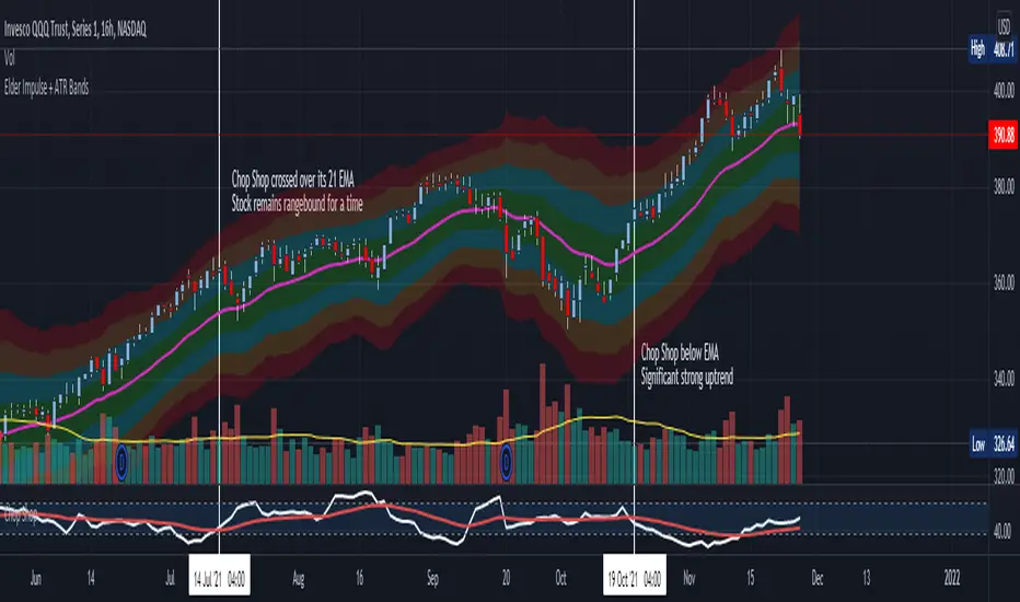
Chop Shop Indicator for Options TradersAs always, this is not financial advice and use at your own risk. Trading is risky and can cost you significant sums of money if you are not careful. Make sure you always have a proper entry and exit plan that includes defining your risk before you enter a trade.
This is for all of you options traders out there who choose to write options and collect premium. Since we seem to be a neglected bunch when it comes to indicators, I figured I would write a script that helps identify when underlyings are in a range and a good time to sell some premium when we are waiting for the next directional setup. This is the choppiness index modified to include a 21-period exponential moving average as a trigger, which I am calling the Chop Shop. The choppiness index , at its most basic, takes a log-scaled version of the summed Average True Range (ATR --- a volatility measurement) and converts it into an oscillator. The higher the oscillator value, the higher level of "chop" the stock is experiencing. This is often referred to as the stock is trading in a range. Most traders are advised to stay out of range trading because it is difficult. However, for an options trader this is an opportune time to collect some premium using bracketed short strike trades such as strangles, straddles, iron condors, or iron butterflies that are profitable when the stock stays rangebound and realizes a drop in volatility .
The indicator is extremely basic. You should look to collect premium and write these types of bracketed trades when Chop Shop crosses over its 21-period EMA . You should look to avoid writing bracketed trades when the Chop Shop trades below its 21-period EMA as this is when a stock is seeing a strong directional movement and can be considered trending. These are usually times when you want to get out of the way of the runaway train and make sure you are on the correct side of the trade or you can quickly get smoked. Use a combination of other indicators to help assist you define the most likely continued direction of the trend and you can then write directional premium trades such as credit spreads, directional Iron Condors, and butterflies to capture this and avoid stepping in front of that moving train.
TASC 2021.11 MADH Moving Average Difference, Hann█ OVERVIEW
Presented here is code for the "Moving Average Difference, Hann" indicator originally conceived by John Ehlers. The code is also published in the November 2021 issue of Trader's Tips by Technical Analysis of Stocks & Commodities (TASC) magazine.
█ CONCEPTS
By employing a Hann windowed finite impulse response filter (FIR), John Ehlers has enhanced the Moving Average Difference (MAD) to provide an oscillator with exceptional smoothness.
Of notable mention, the wave form of MADH resembles Ehlers' "Reverse EMA" Indicator, formerly revealed in the September 2017 issue of TASC. Many variations of the "Reverse EMA" were published in TradingView's Public Library.
█ FEATURES
Three values in the script's "Settings/Inputs" provide control over the oscillators behavior:
• The price source
• A "Short Length" with a default of 8, to manage the lower band edge of the oscillator
• The "Dominant Cycle", originally set at 27, which appears to be a placeholder for an adaptive control mechanism
Two coloring options are provided for the line's fill:
• "ZeroCross", the default, uses the line's position above/below the zero level. This is the mode used in the top version of MADH on this chart.
• "Momentum" uses the line's up/down state, as shown in the bottom version of the indicator on the chart.
█ NOTES
Calculations
The source price is used in two independent Hann windowed FIR filters having two different periods (lengths) of historical observation for calculation, one being a "Short Length" and the other termed "Dominant Cycle". These are then passed to a "rate of change" calculation and then returned by the reusable function. The secret sauce is that a "windowed Hann FIR filter" is superior tp a generic SMA filter, and that ultimately reveals Ehlers' clever enhancement. We'll have to wait and see what ingenuities Ehlers has next to unleash. Stay tuned...
The `madh()` function code was optimized for computational efficiency in Pine, differing visibly from Ehlers' original formula, but yielding the same results as Ehlers' version.
Background
This indicator has a sibling indicator discussed in the "The MAD Indicator, Enhanced" article by Ehlers. MADH is an evolutionary update from the prior MAD indicator code published in the October 2021 issue of TASC.
Sibling Indicators
• Moving Average Difference (MAD)
• Cycle/Trend Analytics
Related Information
• Cycle/Trend Analytics And The MAD Indicator
• The Reverse EMA Indicator
• Hann Window
• ROC
Join TradingView!

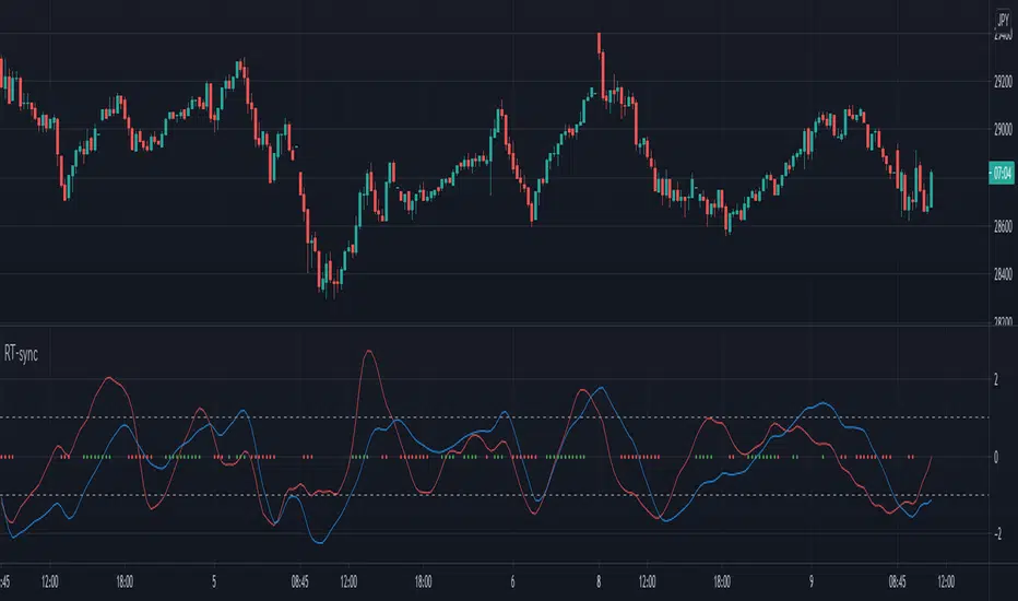
Reflex and Trendflex SyncReflex and Trendflex indicators by John Ehlers .
- Reflex oscillator for market cycles
- Trendflex oscillator for mark trend
The dots indicate that the two oscillators are synchronized.
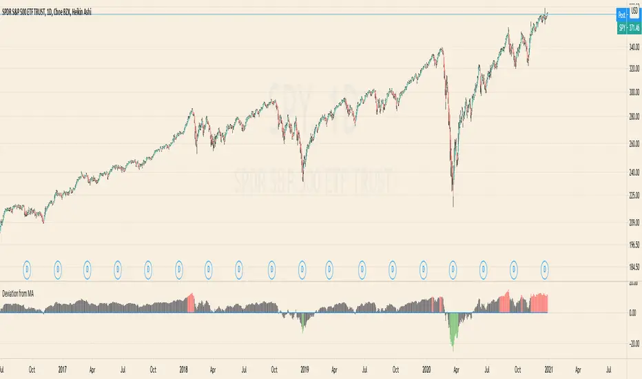
Deviation from MAThe Script calculates the Percentage Deviation to the MA and prints it as an Oscillator.
You can change the following Parameters:
Moving Average Type -> The type of the Moving Average you want to calculate the Deviation on
Length of MA -> The length of the MA
Percentage of Deviation (for Color) -> The Percentage Deviation above or below which the plotted Oscillator is painted in color.
Combo Strategy 123 Reversal & Ergodic TSI This is combo strategies for get a cumulative signal.
First strategy
This System was created from the Book "How I Tripled My Money In The
Futures Market" by Ulf Jensen, Page 183. This is reverse type of strategies.
The strategy buys at market, if close price is higher than the previous close
during 2 days and the meaning of 9-days Stochastic Slow Oscillator is lower than 50.
The strategy sells at market, if close price is lower than the previous close price
during 2 days and the meaning of 9-days Stochastic Fast Oscillator is higher than 50.
Second strategy
r - Length of first EMA smoothing of 1 day momentum 4
s - Length of second EMA smoothing of 1 day smoothing 8
u- Length of third EMA smoothing of 1 day momentum 6
Length of EMA signal line 3
Source of Ergotic TSI Close
This is one of the techniques described by William Blau in his book "Momentum,
Direction and Divergence" (1995). If you like to learn more, we advise you to
read this book. His book focuses on three key aspects of trading: momentum,
direction and divergence. Blau, who was an electrical engineer before becoming
a trader, thoroughly examines the relationship between price and momentum in
step-by-step examples. From this grounding, he then looks at the deficiencies
in other oscillators and introduces some innovative techniques, including a
fresh twist on Stochastics. On directional issues, he analyzes the intricacies
of ADX and offers a unique approach to help define trending and non-trending periods.
WARNING:
- For purpose educate only
- This script to change bars colors.

Combo Strategy 123 Reversal & Ergodic CSI This is combo strategies for get a cumulative signal.
First strategy
This System was created from the Book "How I Tripled My Money In The
Futures Market" by Ulf Jensen, Page 183. This is reverse type of strategies.
The strategy buys at market, if close price is higher than the previous close
during 2 days and the meaning of 9-days Stochastic Slow Oscillator is lower than 50.
The strategy sells at market, if close price is lower than the previous close price
during 2 days and the meaning of 9-days Stochastic Fast Oscillator is higher than 50.
Second strategy
This is one of the techniques described by William Blau in his book
"Momentum, Direction and Divergence" (1995). If you like to learn more,
we advise you to read this book. His book focuses on three key aspects
of trading: momentum, direction and divergence. Blau, who was an electrical
engineer before becoming a trader, thoroughly examines the relationship between
price and momentum in step-by-step examples. From this grounding, he then looks
at the deficiencies in other oscillators and introduces some innovative techniques,
including a fresh twist on Stochastics. On directional issues, he analyzes the
intricacies of ADX and offers a unique approach to help define trending and
non-trending periods.
This indicator plots Ergotic CSI and smoothed Ergotic CSI to filter out noise.
WARNING:
- For purpose educate only
- This script to change bars colors.
OBV with DivergenceAll I did was combine the logic from LazyBear for his OBV Oscillator to regular RSI divergence logic (where I replaced the RSI input to use LazyBear's OBV).
I didn't use any original code! Neither OBV (written by LazyBear) nor DIvergence (author unknown) was written by me. I merely modified the sytax a little to combine them.
Very useful for spotting divergences with OBV oscillator.

Combo Strategy 123 Reversal & Directional Trend Index (DTI) This is combo strategies for get a cumulative signal.
First strategy
This System was created from the Book "How I Tripled My Money In The
Futures Market" by Ulf Jensen, Page 183. This is reverse type of strategies.
The strategy buys at market, if close price is higher than the previous close
during 2 days and the meaning of 9-days Stochastic Slow Oscillator is lower than 50.
The strategy sells at market, if close price is lower than the previous close price
during 2 days and the meaning of 9-days Stochastic Fast Oscillator is higher than 50.
Second strategy
This technique was described by William Blau in his book "Momentum,
Direction and Divergence" (1995). His book focuses on three key aspects
of trading: momentum, direction and divergence. Blau, who was an electrical
engineer before becoming a trader, thoroughly examines the relationship between
price and momentum in step-by-step examples. From this grounding, he then looks
at the deficiencies in other oscillators and introduces some innovative techniques,
including a fresh twist on Stochastics. On directional issues, he analyzes the
intricacies of ADX and offers a unique approach to help define trending and
non-trending periods.
Directional Trend Index is an indicator similar to DM+ developed by Welles Wilder.
The DM+ (a part of Directional Movement System which includes both DM+ and
DM- indicators) indicator helps determine if a security is "trending." William
Blau added to it a zeroline, relative to which the indicator is deemed positive or
negative. A stable uptrend is a period when the DTI value is positive and rising, a
downtrend when it is negative and falling.
WARNING:
- For purpose educate only
- This script to change bars colors.