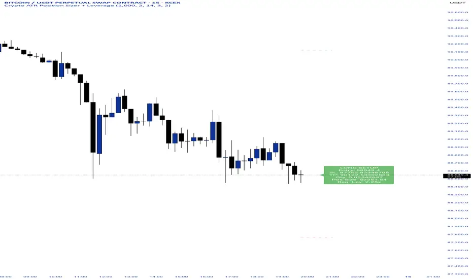
Crypto ATR Position Sizer + LeverageThis indicator is a "heads-up display" for crypto traders who need real time risk management without manually calculating position sizes. It uses Average True Range (ATR) to dynamically place Stop Losses based on current market volatility and automatically calculates the exact position size needed to respect your risk percentage.
Key Features:
Dynamic Risk Management: Stop Loss and Take Profit levels adjust automatically based on market volatility (ATR).
Auto-Position Sizing: Calculates the exact Quantity (in coins) and Position Value (in $) to ensure you never risk more than your defined percentage (e.g., 1% or 2%).
Leverage Calculator: Instantly sees the "Required Leverage" needed to execute the trade size relative to your account balance.
Crypto Precision: Displays up to 8 decimal places, making it compatible with both Bitcoin and low-sat altcoins.
Toggable Direction: Switch between Long and Short biases instantly via the settings menu.
How to Use:
Add the indicator to your chart.
Open Settings and input your Account Balance and Risk %.
Choose your direction (Long or Short) using the checkboxes.
The label will display your Entry, SL, TP, Coin Quantity, and Required Leverage in real-time.
Leverage
DCA Ladder CalculatorThis script is a DCA (Dollar-Cost Averaging) Ladder Calculator with Risk & Leverage Management baked in.
It’s designed for both LONG and SHORT positions, and helps you:
🎯 Strategically scale into positions across multiple entry points
🔐 Control risk exposure via defined capital allocation
⚖️ Utilize leverage responsibly — for efficiency, not destruction
🧮 Visualize risk, stop loss level, and entry distribution
🔁 Adapt to trend reversals or key zones, especially when combined with reversal indicators or higher timeframe signals
🧠 How It Works
This tool takes a capital allocation approach to building a ladder of positions:
1. You define:
- Portfolio value
- Risk per trade (as %)
- Leverage
- Number of DCA levels
- Entry multiplier (e.g. 1x, 2x, 4x...)
2. The script then:
- Calculates total margin to risk = Portfolio × Risk %
- Calculates total leveraged position size = Margin × Leverage
- Distributes entries according to exponential weights (1x, 2x, 4x...), totaling 7 for 3 levels
- Calculates per-entry:
- Entry price (based on price zone spacing)
- Multiplier
- Exact margin per entry
- Leverage per entry (margin × leverage)
- Computes:
- Average entry price (margin-weighted)
- Approximate stop loss level based on recent ATR and price structure
- % drawdown to SL
- Total margin and position size
3. Displays all this in a clean on-chart table.
📈 How to Use It
1. Apply the indicator to a chart (default: 1D — ideal for clean zones).
2. Configure your:
- Portfolio Value (total trading capital)
- Risk per Trade (%) (your acceptable loss)
- Leverage (exchange or strategy-based)
- DCA Levels (e.g. 3 = anchor + 2 entries)
- Multiplier (typically 2.0 for doubling)
3. Choose LONG or SHORT mode depending on direction.
4. The table will show:
- Entry price ladder
- Margin used per entry
- Total position size
- Approx. stop loss (where your full risk is defined)
Use in conjunction with price action, S/R zones, trendline breaks, volume divergence, or reversal indicators.
✅ Best Practices for Using This Tool
- Leverage is a tool, not a weapon. Use it to scale smartly — not recklessly.
- Use fewer, higher-conviction entries. Don’t blindly ladder; combine with price structure and signals.
- Stick to your risk percent. Never risk more than you can afford to lose. Let this calculator enforce discipline.
- Combine with other confirmation tools, like RSI divergence, momentum shifts, OB zones, etc.
- Avoid martingale-style over-exposure. This is not a gambling tool — it’s for capital efficiency.
🛡️ What This Tool Does NOT Do
- This is not a trade signal indicator.
- It does not place trades or auto-manage positions.
- It does not replace personal responsibility or strategy — it's a tool to help apply structure.
⚠️ Disclaimer
This script is for educational and informational purposes only.
It does not constitute financial advice, nor is it a recommendation to buy or sell any financial instrument.
Always consult a licensed financial advisor before making investment decisions.
Use of leverage involves high risk and can lead to substantial losses.
The author and publisher assume no liability for any trading losses resulting from use of this script.

Position Size Calculator + Live R/R Panel — SMC/ICT (@PueblaATH)Position Size + Live R/R Panel — SMC/ICT (@PueblaATH)
Position Size + Live R/R Panel — SMC/ICT (@PueblaATH) is a professional-grade risk management and execution module built for Smart Money Concepts (SMC) and ICT Traders who require accurate, repeatable, institution-style trade planning.
This tool delivers precise position sizing, R:R modeling, leverage and margin projections, fee-adjusted PnL outcomes, and real-time execution metrics—all directly on the chart. Optimized for crypto, forex, and futures, it provides scalpers, day traders, and swing traders with the clarity needed to execute high-quality trades with confidence and consistency.
What the Indicator Does
Institutional Position Sizing Engine
Calculates position size based on account balance, % risk, and SL distance.
Supports custom minimum lot size rounding across crypto, FX, indices, and derivatives.
Intelligent direction logic (Auto / Long / Short) based on SMC/ICT structure.
Advanced Risk/Reward & Profit Modeling
Real-time R:R ratio using actual rounded position size.
Live PnL readout that updates with price movements.
Gross & net profit projections with full fee deduction.
Execution Planning with Draggable Levels
Entry, SL, and TP levels fully draggable for fast scenario modeling.
Automatic projected lines backward/forward with clean label alignment.
TP and SL tags include % movement from Entry, ideal for SMC/ICT journaling.
Precise modeling of real exchange fee structures
Maker fee per side
Taker fee per side
Mixed fee modes (Maker entry, Taker exit, Average, etc.)
Leverage & Margin Forecasting
Margin requirements displayed for 3 customizable leverage settings.
Helps traders understand capital commitment before executing the trade.
Useful for futures, crypto perps, and CFD setups.
Clean HUD Panel for Rapid Decision-Making
A full professional trading panel displays:
Target & actual risk
Position size
Entry / SL / TP
TP/SL percentage distance
Gross profit
Net profit (after fees)
Fees @ TP and @ SL
Live PnL
Margin requirements
Optimized for SMC & ICT Workflows
Perfect for traders using:
Breakers, FVGs, OBs
Liquidity sweeps
Session models
Precision entries (OTE, Displacement, Rebalancing)
Leverage-based execution (crypto perps, futures)
How to Use It
Attach the indicator to your chart.
Set account balance, risk %, fee model, and leverage presets.
Drag Entry, SL, and TP to shape the setup.
View instant calculations of: Position size; R:R; Net PnL after fees; Margin required
Use it as your pre-trade checklist & execution model.
Originality & Credits
This script is an original creation by @PueblaATH, released under the MPL 2.0 license.
It does not copy, modify, or repackage any existing TradingView code.
All logic—including the fee engine, margin calculator, responsive HUD, dynamic risk model, and visual execution system—is authored specifically for this indicator.

Multi-Mode Grid StrategyGrid Strategy (SIMPLE)
█ Overview
This script is a system trading tool designed to generate cash flow from market volatility without relying on short-term directional predictions. It operates on the principle of Grid Trading , creating a mesh of buy and sell orders within a user-defined price range.
The strategy automates the process of "buying the dip" and "selling the bounce" repeatedly. It is most effective in sideways markets or during accumulation phases where the price oscillates within a specific channel.
█ TRADING MINDSET & SETUP GUIDE
To use this tool effectively, you must shift your perspective from "Sniper" (trying to hit the perfect entry) to "Manager" (managing a zone). Here is the required mindset for setting up this strategy:
Shift from Prediction to Range Definition
Don't ask: "Will the price go up or down tomorrow?"
Ask instead: "What is the price range the asset is unlikely to break out of in the coming weeks?"
Your primary job is to define the Grid Top Price (Ceiling) and Grid Bottom Price (Floor). As long as the price stays within this "Arena," the strategy will continue to execute trades.
Embrace Volatility as Fuel
For a trend follower, chop/sideways action is a nightmare. For a Grid Trader, it is fuel. Every time the price crosses a grid line down, it builds inventory. Every time it crosses back up, it realizes profit. You want the price to wiggle as much as possible within your defined boundaries.
Capital Allocation & Survivability
The biggest risk in grid trading is the price crashing below your Grid Bottom Price .
Mindset Check: Before launching, assume the price WILL drop to your bottom price immediately. Can your account handle that drawdown?
The script includes leverage and capital percentage inputs to help you size your position correctly. Never allocate 100% of your capital to a tight range without understanding the liquidation risk.
█ HOW IT WORKS
Grid Construction:
The script divides the space between your Upper Border and Lower Border into specific levels based on the Grid Quantity .
- Arithmetic: Equal spacing between lines (Standard).
- Geometric: Spacing based on mathematical ratios (useful for wider ranges).
Execution Logic:
- Entry: When price crosses below a grid line, a Long position is opened.
- Exit: When price bounces back up by a specific number of grid levels (defined by "Distance of TP"), the specific position is closed for a profit.
Time & Backtesting:
You can set specific Start and End Times . This allows you to backtest how the grid would have performed during specific historical volatility events before deploying it on live markets.
█ VISUALIZATION DASHBOARD
To keep you informed without cluttering the chart, the script features an information table at the bottom right:
Cash Out: Total realized profit booked into the account.
Open Position: How many grid levels are currently active (holding bags) vs. total levels.
Open Trade: The current floating P/L of held positions (Unrealized).
Max Drawdown: The deepest drawdown the strategy experienced during the test period.
RISK DISCLAIMER
Grid trading involves significant risk, particularly in strong trending markets that break out of your range against your position. This strategy does not use a stop-loss per trade; it relies on the user defining a safe "Bottom Price" and allocating capital accordingly. Past performance in backtesting does not guarantee future results. This script is a tool for execution and analysis, not financial advice.

[Saga Trading] Liquidation Leverages ProSaga Trading – Liquidation Leverages Pro
Liquidation Leverages Pro is a powerful TradingView indicator designed to map the real-time liquidation levels of traders using leverage from 1x up to 100x on Bitget futures. By calculating the theoretical liquidation price of each leverage tier, the tool reveals where the majority of leveraged positions become vulnerable — and where Market Makers have incentives to drive price.
The indicator visually displays these liquidation levels directly on the chart, allowing traders to instantly identify liquidity pools, liquidation clusters, stop-hunt zones, and high-risk areas. Each leverage tier can be toggled on or off, and clusters of overlapping liquidation levels are automatically highlighted to expose areas where forced liquidations could trigger sharp market moves.
This tool provides deep insight into the behavior and positioning of the majority, helping traders understand where the next engineered move is most likely to occur. When combined with order-flow tools made by Saga Trading such as Aggregated CVD Pro, Synthetic OrderBook, and Open Interest, Liquidation Leverages Pro becomes an essential component of a full liquidity-based trading system.
Whether you scalp, swing trade, or analyze derivatives, this indicator gives you a decisive advantage by showing exactly where the market is most fragile — and where the next cascade can begin.

Volatility-Targeted Momentum Portfolio [BackQuant]Volatility-Targeted Momentum Portfolio
A complete momentum portfolio engine that ranks assets, targets a user-defined volatility, builds long, short, or delta-neutral books, and reports performance with metrics, attribution, Monte Carlo scenarios, allocation pie, and efficiency scatter plots. This description explains the theory and the mechanics so you can configure, validate, and deploy it with intent.
Table of contents
What the script does at a glance
Momentum, what it is, how to know if it is present
Volatility targeting, why and how it is done here
Portfolio construction modes: Long Only, Short Only, Delta Neutral
Regime filter and when the strategy goes to cash
Transaction cost modelling in this script
Backtest metrics and definitions
Performance attribution chart
Monte Carlo simulation
Scatter plot analysis modes
Asset allocation pie chart
Inputs, presets, and deployment checklist
Suggested workflow
1) What the script does at a glance
Pulls a list of up to 15 tickers, computes a simple momentum score on each over a configurable lookback, then volatility-scales their bar-to-bar return stream to a target annualized volatility.
Ranks assets by raw momentum, selects the top 3 and bottom 3, builds positions according to the chosen mode, and gates exposure with a fast regime filter.
Accumulates a portfolio equity curve with risk and performance metrics, optional benchmark buy-and-hold for comparison, and a full alert suite.
Adds visual diagnostics: performance attribution bars, Monte Carlo forward paths, an allocation pie, and scatter plots for risk-return and factor views.
2) Momentum: definition, detection, and validation
Momentum is the tendency of assets that have performed well to continue to perform well, and of underperformers to continue underperforming, over a specific horizon. You operationalize it by selecting a horizon, defining a signal, ranking assets, and trading the leaders versus laggards subject to risk constraints.
Signal choices . Common signals include cumulative return over a lookback window, regression slope on log-price, or normalized rate-of-change. This script uses cumulative return over lookback bars for ranking (variable cr = price/price - 1). It keeps the ranking simple and lets volatility targeting handle risk normalization.
How to know momentum is present .
Leaders and laggards persist across adjacent windows rather than flipping every bar.
Spread between average momentum of leaders and laggards is materially positive in sample.
Cross-sectional dispersion is non-trivial. If everything is flat or highly correlated with no separation, momentum selection will be weak.
Your validation should include a diagnostic that measures whether returns are explained by a momentum regression on the timeseries.
Recommended diagnostic tool . Before running any momentum portfolio, verify that a timeseries exhibits stable directional drift. Use this indicator as a pre-check: It fits a regression to price, exposes slope and goodness-of-fit style context, and helps confirm if there is usable momentum before you force a ranking into a flat regime.
3) Volatility targeting: purpose and implementation here
Purpose . Volatility targeting seeks a more stable risk footprint. High-vol assets get sized down, low-vol assets get sized up, so each contributes more evenly to total risk.
Computation in this script (per asset, rolling):
Return series ret = log(price/price ).
Annualized volatility estimate vol = stdev(ret, lookback) * sqrt(tradingdays).
Leverage multiplier volMult = clamp(targetVol / vol, 0.1, 5.0).
This caps sizing so extremely low-vol assets don’t explode weight and extremely high-vol assets don’t go to zero.
Scaled return stream sr = ret * volMult. This is the per-bar, risk-adjusted building block used in the portfolio combinations.
Interpretation . You are not levering your account on the exchange, you are rescaling the contribution each asset’s daily move has on the modeled equity. In live trading you would reflect this with position sizing or notional exposure.
4) Portfolio construction modes
Cross-sectional ranking . Assets are sorted by cr over the chosen lookback. Top and bottom indices are extracted without ties.
Long Only . Averages the volatility-scaled returns of the top 3 assets: avgRet = mean(sr_top1, sr_top2, sr_top3). Position table shows per-asset leverages and weights proportional to their current volMult.
Short Only . Averages the negative of the volatility-scaled returns of the bottom 3: avgRet = mean(-sr_bot1, -sr_bot2, -sr_bot3). Position table shows short legs.
Delta Neutral . Long the top 3 and short the bottom 3 in equal book sizes. Each side is sized to 50 percent notional internally, with weights within each side proportional to volMult. The return stream mixes the two sides: avgRet = mean(sr_top1,sr_top2,sr_top3, -sr_bot1,-sr_bot2,-sr_bot3).
Notes .
The selection metric is raw momentum, the execution stream is volatility-scaled returns. This separation is deliberate. It avoids letting volatility dominate ranking while still enforcing risk parity at the return contribution stage.
If everything rallies together and dispersion collapses, Long Only may behave like a single beta. Delta Neutral is designed to extract cross-sectional momentum with low net beta.
5) Regime filter
A fast EMA(12) vs EMA(21) filter gates exposure.
Long Only active when EMA12 > EMA21. Otherwise the book is set to cash.
Short Only active when EMA12 < EMA21. Otherwise cash.
Delta Neutral is always active.
This prevents taking long momentum entries during obvious local downtrends and vice versa for shorts. When the filter is false, equity is held flat for that bar.
6) Transaction cost modelling
There are two cost touchpoints in the script.
Per-bar drag . When the regime filter is active, the per-bar return is reduced by fee_rate * avgRet inside netRet = avgRet - (fee_rate * avgRet). This models proportional friction relative to traded impact on that bar.
Turnover-linked fee . The script tracks changes in membership of the top and bottom baskets (top1..top3, bot1..bot3). The intent is to charge fees when composition changes. The template counts changes and scales a fee by change count divided by 6 for the six slots.
Use case: increase fee_rate to reflect taker fees and slippage if you rebalance every bar or trade illiquid assets. Reduce it if you rebalance less often or use maker orders.
Practical advice .
If you rebalance daily, start with 5–20 bps round-trip per switch on liquid futures and adjust per venue.
For crypto perp microcaps, stress higher cost assumptions and add slippage buffers.
If you only rotate on lookback boundaries or at signals, use alert-driven rebalances and lower per-bar drag.
7) Backtest metrics and definitions
The script computes a standard set of portfolio statistics once the start date is reached.
Net Profit percent over the full test.
Max Drawdown percent, tracked from running peaks.
Annualized Mean and Stdev using the chosen trading day count.
Variance is the square of annualized stdev.
Sharpe uses daily mean adjusted by risk-free rate and annualized.
Sortino uses downside stdev only.
Omega ratio of sum of gains to sum of losses.
Gain-to-Pain total gains divided by total losses absolute.
CAGR compounded annual growth from start date to now.
Alpha, Beta versus a user-selected benchmark. Beta from covariance of daily returns, Alpha from CAPM.
Skewness of daily returns.
VaR 95 linear-interpolated 5th percentile of daily returns.
CVaR average of the worst 5 percent of daily returns.
Benchmark Buy-and-Hold equity path for comparison.
8) Performance attribution
Cumulative contribution per asset, adjusted for whether it was held long or short and for its volatility multiplier, aggregated across the backtest. You can filter to winners only or show both sides. The panel is sorted by contribution and includes percent labels.
9) Monte Carlo simulation
The panel draws forward equity paths from either a Normal model parameterized by recent mean and stdev, or non-parametric bootstrap of recent daily returns. You control the sample length, number of simulations, forecast horizon, visibility of individual paths, confidence bands, and a reproducible seed.
Normal uses Box-Muller with your seed. Good for quick, smooth envelopes.
Bootstrap resamples realized returns, preserving fat tails and volatility clustering better than a Gaussian assumption.
Bands show 10th, 25th, 75th, 90th percentiles and the path mean.
10) Scatter plot analysis
Four point-cloud modes, each plotting all assets and a star for the current portfolio position, with quadrant guides and labels.
Risk-Return Efficiency . X is risk proxy from leverage, Y is expected return from annualized momentum. The star shows the current book’s composite.
Momentum vs Volatility . Visualizes whether leaders are also high vol, a cue for turnover and cost expectations.
Beta vs Alpha . X is a beta proxy, Y is risk-adjusted excess return proxy. Useful to see if leaders are just beta.
Leverage vs Momentum . X is volMult, Y is momentum. Shows how volatility targeting is redistributing risk.
11) Asset allocation pie chart
Builds a wheel of current allocations.
Long Only, weights are proportional to each long asset’s current volMult and sum to 100 percent.
Short Only, weights show the short book as positive slices that sum to 100 percent.
Delta Neutral, 50 percent long and 50 percent short books, each side leverage-proportional.
Labels can show asset, percent, and current leverage.
12) Inputs and quick presets
Core
Portfolio Strategy . Long Only, Short Only, Delta Neutral.
Initial Capital . For equity scaling in the panel.
Trading Days/Year . 252 for stocks, 365 for crypto.
Target Volatility . Annualized, drives volMult.
Transaction Fees . Per-bar drag and composition change penalty, see the modelling notes above.
Momentum Lookback . Ranking horizon. Shorter is more reactive, longer is steadier.
Start Date . Ensure every symbol has data back to this date to avoid bias.
Benchmark . Used for alpha, beta, and B&H line.
Diagnostics
Metrics, Equity, B&H, Curve labels, Daily return line, Rolling drawdown fill.
Attribution panel. Toggle winners only to focus on what matters.
Monte Carlo mode with Normal or Bootstrap and confidence bands.
Scatter plot type and styling, labels, and portfolio star.
Pie chart and labels for current allocation.
Presets
Crypto Daily, Long Only . Lookback 25, Target Vol 50 percent, Fees 10 bps, Regime filter on, Metrics and Drawdown on. Monte Carlo Bootstrap with Recent 200 bars for bands.
Crypto Daily, Delta Neutral . Lookback 25, Target Vol 50 percent, Fees 15–25 bps, Regime filter always active for this mode. Use Scatter Risk-Return to monitor efficiency and keep the star near upper left quadrants without drifting rightward.
Equities Daily, Long Only . Lookback 60–120, Target Vol 15–20 percent, Fees 5–10 bps, Regime filter on. Use Benchmark SPX and watch Alpha and Beta to keep the book from becoming index beta.
13) Suggested workflow
Universe sanity check . Pick liquid tickers with stable data. Thin assets distort vol estimates and fees.
Check momentum existence . Run on your timeframe. If slope and fit are weak, widen lookback or avoid that asset or timeframe.
Set risk budget . Choose a target volatility that matches your drawdown tolerance. Higher target increases turnover and cost sensitivity.
Pick mode . Long Only for bull regimes, Short Only for sustained downtrends, Delta Neutral for cross-sectional harvesting when index direction is unclear.
Tune lookback . If leaders rotate too often, lengthen it. If entries lag, shorten it.
Validate cost assumptions . Increase fee_rate and stress Monte Carlo. If the edge vanishes with modest friction, refine selection or lengthen rebalance cadence.
Run attribution . Confirm the strategy’s winners align with intuition and not one unstable outlier.
Use alerts . Enable position change, drawdown, volatility breach, regime, momentum shift, and crash alerts to supervise live runs.
Important implementation details mapped to code
Momentum measure . cr = price / price - 1 per symbol for ranking. Simplicity helps avoid overfitting.
Volatility targeting . vol = stdev(log returns, lookback) * sqrt(tradingdays), volMult = clamp(targetVol / vol, 0.1, 5), sr = ret * volMult.
Selection . Extract indices for top1..top3 and bot1..bot3. The arrays rets, scRets, lev_vals, and ticks_arr track momentum, scaled returns, leverage multipliers, and display tickers respectively.
Regime filter . EMA12 vs EMA21 switch determines if the strategy takes risk for Long or Short modes. Delta Neutral ignores the gate.
Equity update . Equity multiplies by 1 + netRet only when the regime was active in the prior bar. Buy-and-hold benchmark is computed separately for comparison.
Tables . Position tables show current top or bottom assets with leverage and weights. Metric table prints all risk and performance figures.
Visualization panels . Attribution, Monte Carlo, scatter, and pie use the last bars to draw overlays that update as the backtest proceeds.
Final notes
Momentum is a portfolio effect. The edge comes from cross-sectional dispersion, adequate risk normalization, and disciplined turnover control, not from a single best asset call.
Volatility targeting stabilizes path but does not fix selection. Use the momentum regression link above to confirm structure exists before you size into it.
Always test higher lag costs and slippage, then recheck metrics, attribution, and Monte Carlo envelopes. If the edge persists under stress, you have something robust.

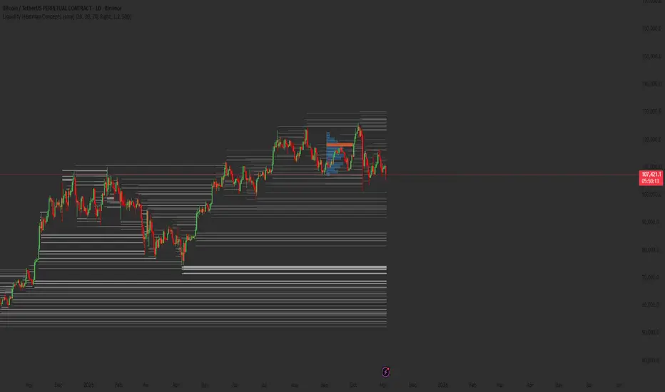
Liquidity Heatmap Concepts [sma] Overview
Liquidity Heatmap Concepts is a sophisticated visualization tool that maps potential liquidation zones for leveraged positions across multiple timeframes. It calculates and displays where high-volume liquidations might occur at various leverage levels (25x, 50x, 100x, 150x), helping traders identify potential support/resistance zones created by cascading liquidations. Additionally, it includes a quarterly volume profile to show historical price distribution and Point of Control levels.
### Volume-Based Trigger System
Lines are only drawn when volume exceeds a threshold:
1. Calculates 14-period simple moving average of volume
2. Applies configurable multiplier (default 1.2x) to determine significance
3. Only plots liquidation levels when current volume > (Volume SMA × Multiplier)
4. This filters out low-volume noise and focuses on meaningful zones
### Visual Intensity System
The indicator uses a gradient coloring system based on relative volume:
- **Peak Volume (White)**: When current bar has maximum volume in the dataset
- Line width: 3 pixels
- Brightest color intensity
- **Above Average Volume**: Volume exceeds average but isn't peak
- Line width: 2 pixels
- Medium color intensity
- **Standard Volume**: Exceeds threshold but below average
- Line width: 1 pixel
- Base color intensity
### Line Extension & Management
- Lines extend horizontally to the right until price crosses them
- Automatic cleanup removes lines after maximum count (default 500)
- Lines persist until invalidated by price action crossing the level
- Oldest lines are removed first when limit is reached
### Quarterly Volume Profile
An optional fixed-range volume profile that:
1. **Automatic Quarter Detection**: Identifies Q1 (Jan-Mar), Q2 (Apr-Jun), Q3 (Jul-Sep), Q4 (Oct-Dec)
2. **Price Distribution Analysis**: Divides the quarter's price range into configurable rows (default 20)
3. **Volume Aggregation**: Accumulates volume at each price level throughout the quarter
4. **POC Identification**: Highlights the price level with highest volume (Point of Control)
5. **Value Area**: Shows the price range containing 70% (configurable) of total volume
6. **Profile Drawing**: At the start of each new quarter, draws the previous quarter's profile as horizontal bars
The volume profile can be positioned on either left or right side of the quarter range with adjustable width.
## Key Features
- **Multi-Leverage Display**: Toggle between 25x, 50x, 100x, and 150x leverage levels independently
- **Dual Side Tracking**: Separate visualization for long and short liquidation zones
- **Volume-Weighted Importance**: Visual intensity correlates with volume significance
- **Gradient Coloring**: Color intensity reflects relative volume magnitude
- **Smart Line Management**: Automatic cleanup prevents chart clutter
- **Historical Context**: Quarterly volume profile shows where price spent most time
- **Fully Customizable**: All colors, thresholds, and display options are adjustable
- **HD Mode**: Uses absolute volume for more precise visualization
## Parameters
### Leverage Selection
- **25x, 50x, 100x, 150x Toggles**: Enable/disable specific leverage levels
- Each level can be controlled independently
### Volume Configuration
- **Minimum Volume Multiplier** (default 1.2): Threshold above volume SMA to trigger lines
- Higher values = fewer but more significant levels
- Lower values = more levels but increased noise
### Advanced Settings
- **Maximum Lines** (default 500, range 50-500): Memory management limit
- Controls how many historical liquidation lines are maintained
### Quarterly Volume Profile
- **Show Previous Q Volume Profile** (default on): Toggle profile visibility
- **Number of Rows** (default 20, range 10-50): Price distribution granularity
- **Profile Width** (default 30%): Visual width as percentage of quarter range
- **Value Area** (default 70%): Percentage of volume for value area calculation
- **Position** (Left/Right): Profile placement relative to quarter
- **Show Values** (default off): Display POC volume label
- **Colors**: Customizable base and POC colors
### Color Customization
- **Long Colors**: Individual colors for each leverage level (25x, 50x, 100x, 150x)
- **Short Colors**: Separate color scheme for short liquidation zones
- **VP Colors**: Base color and POC highlight color for volume profile
## Interpretation
### Liquidation Clusters
- **Dense Line Areas**: Multiple overlapping liquidation levels suggest strong magnetic zones
- **High-Volume Lines**: Brighter/thicker lines indicate more significant potential liquidations
- **Line Breaks**: Price crossing multiple liquidation lines may trigger cascade effects
### Trading Applications
- **Support/Resistance**: Liquidation clusters often act as temporary support/resistance
- **Stop Hunt Zones**: Areas where price may spike to trigger liquidations before reversing
- **Momentum Acceleration**: Breaking through dense clusters can indicate strong directional moves
- **Risk Management**: Avoid placing stops directly at obvious liquidation levels
### Volume Profile Usage
- **POC (Point of Control)**: Price level with highest volume - often acts as strong support/resistance
- **Value Area**: Where most trading activity occurred - indicates fair value range
- **Profile Shape**:
- Balanced profile (bell curve) = ranging market
- Skewed profile = trending market with acceptance at extremes
- **Profile Gaps**: Low volume areas suggest price may move quickly through these zones
### Combined Analysis
- Liquidation lines near quarterly POC create extra-strong zones
- Price returning to value area from outside often finds support/resistance
- Liquidation clusters at value area edges suggest potential reversal points
## Technical Implementation
This indicator features:
- **Custom Type Structures**: Uses type definitions for organized data storage
- `BarData`: Stores OHLCV and index information
- `LiquidityBin`: Manages arrays of line objects for each leverage level
- `VolumeProfileData`: Handles profile boxes, labels, and range data
- **Dynamic Line Objects**: Creates, updates, and deletes line primitives programmatically
- **Array-Based History**: Maintains volume history for gradient calculations
- **Intelligent Cleanup**: Automatic memory management prevents performance degradation
- **Mathematical Precision**: Leverage-based liquidation formulas ensure accurate price levels
- **Quarterly Aggregation**: Efficient volume accumulation with automatic period detection
- **Box Drawing System**: Dynamic profile visualization using box primitives
## Originality Statement
This indicator presents a unique approach to liquidity visualization:
- Implements leverage-specific liquidation price calculations based on mathematical formulas
- Uses volume-weighted gradient coloring system that adapts to relative volume significance
- Combines real-time liquidation mapping with historical volume profile analysis
- Features intelligent line lifecycle management with automatic extension and cleanup
- Integrates quarterly volume profile with configurable value area and POC detection
- Employs multi-layer visual hierarchy (line width + color intensity) for information density
- Uses custom data structures to efficiently manage hundreds of line objects simultaneously
The combination of mathematical liquidation pricing, volume-based filtering, gradient visualization, and quarterly volume distribution creates a comprehensive liquidity analysis tool.
## Best Practices
- Use on liquid markets (major cryptocurrencies, forex pairs) for best accuracy
- Lower timeframes (1m-15m) for day trading and scalping
- Higher timeframes (1h-4h) for swing trading context
- Combine with volume profile to identify high-probability reversal zones
- Watch for price reactions when approaching dense liquidation clusters
- Increase volume multiplier in choppy markets to reduce noise
- Reduce maximum lines on lower timeframes to maintain performance
- Use quarterly volume profile to understand longer-term fair value
## Important Notes
- Liquidation prices are estimates based on leverage ratios
- Actual exchange liquidation prices may vary due to:
- Maintenance margin requirements
- Mark price vs last price calculations
- Individual exchange liquidation engines
- Insurance fund mechanisms
- This tool shows potential zones, not guaranteed liquidation prices
- Volume profile resets each quarter automatically
---
Works on all timeframes and asset classes. Designed for crypto/forex leverage markets. For educational purposes only. Not financial advice.
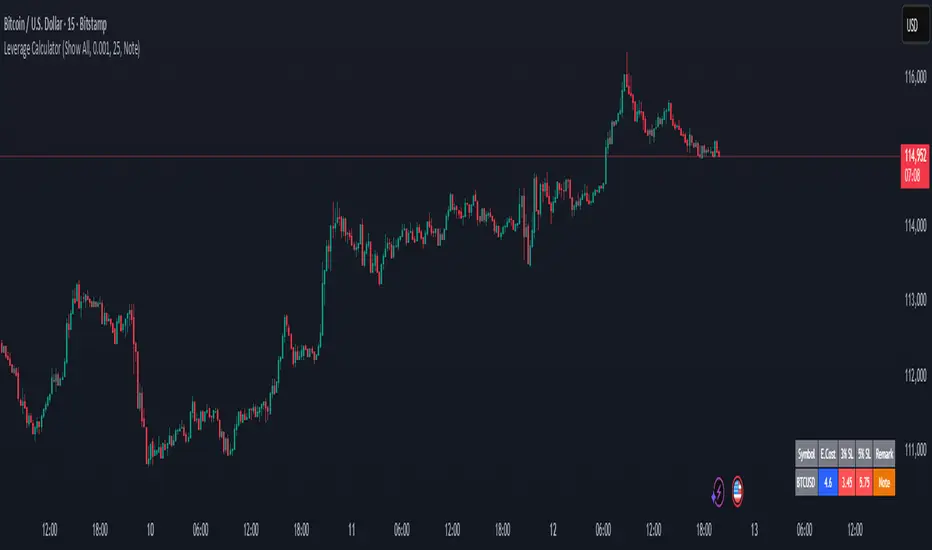
Margin Cost Calculator Screener - Taylor V1.2# Leverage Position Cost Calculator & Stop Lose Cost Screener #
Designed to provide traders with crucial insights into their leveraged positions directly on the TradingView chart.
Key Features:
> Dynamic Display: Choose to view only the estimated entry cost, or a comprehensive overview including potential losses at specific stop-loss levels, and a custom remark.
> Contract Size Input: Easily specify the contract size for your trades.
> Leverage Level Input: Set your desired leverage level, with helpful tooltips explaining the margin requirements for various leverage ratios (e.g., 25x, 10x, 5x) and an included fee estimate.
> Cost Calculation: Accurately calculates the estimated entry cost for your position based on the current market price, contract size, and leverage.
> Stop-Loss Projections: It projects potential losses for stop-loss orders set at 3% and 5% below the entry price, helping you manage risk effectively.
> Clear Table Visualization: All calculated data is presented in a clean, organized table anchored to the bottom-left of your chart, making it easy to reference at a glance.
> Symbol Identification: Automatically displays the short ticker symbol for the asset you are analyzing.
This tool is invaluable for traders who utilize leverage and need a quick, visual way to understand their financial exposure and potential outcomes before entering or managing a trade.
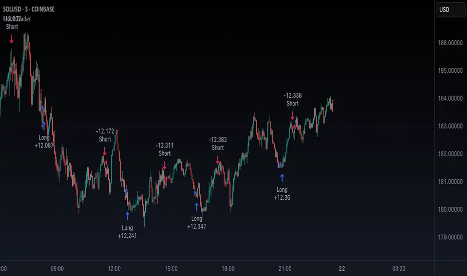
Stoch TraderSimple example strategy that has greater than 60% win rate on 1m, 3m, and 5m views. Using something as simple as this with leverage can produce decent returns within 15-30min. It's also very easy to lose money doing this.
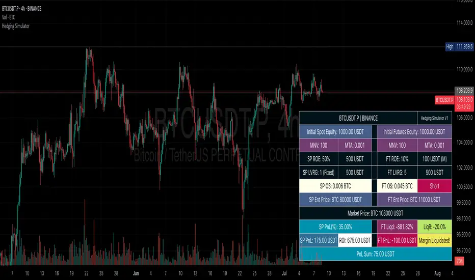
Hedging SimulatorHedging Simulator
The Hedging Simulator is a straightforward hedging tool designed to simulate potential profit and loss outcomes from combined Spot and Futures positions in the cryptocurrency market.
Users can define their equity allocation separately for both spot and futures, allowing for flexible and realistic scenario modelling.
The tool also incorporates MNV (Minimum Notional Value) and MTA (Minimum Trade Amount) parameters to estimate order sizes based on symbol-specific trading rules set by exchanges. While the results may differ slightly from actual exchange calculations, the simulator aims to provide a close approximation for general understanding.
📌Note: Crypto-Only - This tool is designed specifically for cryptocurrency trading and is not intended for use with traditional financial instruments.
Entry Price: Users can input custom entry prices for both spot and futures trades to simulate from specific market positions.
Live Price: The entry price fields for both spot and futures support Live Price based on the currently viewed symbol on your chart.
📌Note: In the real market, spot and futures prices are not always identical—there can be a price gap between them. While the difference is typically small, it's important to understand that the live price shown is only for rough estimation purposes and may not reflect the exact trading price on your chosen exchange.
Expecting Market Price: This represents the projected or target price to simulate potential profit and loss across the hedged position based on market movement.
📌Note: Profit and loss calculations exclude all trading fees. Actual results in live markets may vary due to fees, slippage, and exchange rules.
Feedback: If you notice any bugs, errors on calculation, or have suggestions for better calculations or new features, feel free to share your thoughts. Your feedback helps improve the tool and will be considered for future updates.
⚠️ Disclaimer: This simulator is intended for educational and illustrative purposes only. It does not constitute financial advice or guarantee trading results. Market conditions may vary, and all trading carries inherent risks. Users are solely responsible for any decisions made based on this tool and bear full responsibility for their own trading outcomes.
SAFE Leverage Pro x50Safe Leverage Pro x50 — Safe leverage based on timeframes
Description:
Safe Leverage Pro x50 is an indicator designed to help traders choose prudent and realistic leverage, tailored to the timeframe being traded and the asset chosen.
Based on rigorous statistical research, this indicator provides a visual recommendation of the maximum typical leverage by timeframe and automatically suggests a more conservative value (by default, half) for trading with greater peace of mind and risk control.
* The goal is not for the indicator to make decisions for you, but rather to support your pre-defined entry strategies, allowing you to clearly understand how much leverage you can use without compromising your account against normal price fluctuations.
*The indicator does not calculate based on real-time volatility or ATR, but rather relies on statistical historical patterns obtained by analyzing price behavior after entry, differentiating between average movements in long and short entries by timeframe.
Important: Before following the recommendations of this indicator, check the maximum leverage your broker or exchange allows for the asset you are trading, as it can vary significantly between platforms.
* Philosophy behind the indicator:
This project arises as a response to the simplistic discourse that condemns leverage without distinguishing nuances.
Leverage is not intrinsically bad. What is dangerous is leveraging without method, without awareness, and without risk management.
Safe Leverage Pro x50 is designed to change that narrative:
** It's not about whether or not to use leverage, but when, how much, and how to use it intelligently.

TitanGrid L/S SuperEngineTitanGrid L/S SuperEngine
Experimental Trend-Aligned Grid Signal Engine for Long & Short Execution
🔹 Overview
TitanGrid is an advanced, real-time signal engine built around a tactical grid structure.
It manages Long and Short trades using trend-aligned entries, layered scaling, and partial exits.
Unlike traditional strategy() -based scripts, TitanGrid runs as an indicator() , but includes its own full internal simulation engine.
This allows it to track capital, equity, PnL, risk exposure, and trade performance bar-by-bar — effectively simulating a custom backtest, while remaining compatible with real-time alert-based execution systems.
The concept was born from the fusion of two prior systems:
Assassin’s Grid (grid-based execution and structure) + Super 8 (trend-filtering, smart capital logic), both developed under the AssassinsGrid framework.
🔹 Disclaimer
This is an experimental tool intended for research, testing, and educational use.
It does not provide guaranteed outcomes and should not be interpreted as financial advice.
Use with demo or simulated accounts before considering live deployment.
🔹 Execution Logic
Trend direction is filtered through a custom SuperTrend engine. Once confirmed:
• Long entries trigger on pullbacks, exiting progressively as price moves up
• Short entries trigger on rallies, exiting as price declines
Grid levels are spaced by configurable percentage width, and entries scale dynamically.
🔹 Stop Loss Mechanism
TitanGrid uses a dual-layer stop system:
• A static stop per entry, placed at a fixed percentage distance matching the grid width
• A trend reversal exit that closes the entire position if price crosses the SuperTrend in the opposite direction
Stops are triggered once per cycle, ensuring predictable and capital-aware behavior.
🔹 Key Features
• Dual-side grid logic (Long-only, Short-only, or Both)
• SuperTrend filtering to enforce directional bias
• Adjustable grid spacing, scaling, and sizing
• Static and dynamic stop-loss logic
• Partial exits and reset conditions
• Webhook-ready alerts (browser-based automation compatible)
• Internal simulation of equity, PnL, fees, and liquidation levels
• Real-time dashboard for full transparency
🔹 Best Use Cases
TitanGrid performs best in structured or mean-reverting environments.
It is especially well-suited to assets with the behavioral profile of ETH — reactive, trend-intraday, and prone to clean pullback formations.
While adaptable to multiple timeframes, it shows strongest performance on the 15-minute chart , offering a balance of signal frequency and directional clarity.
🔹 License
Published under the Mozilla Public License 2.0 .
You are free to study, adapt, and extend this script.
🔹 Panel Reference
The real-time dashboard displays performance metrics, capital state, and position behavior:
• Asset Type – Automatically detects the instrument class (e.g., Crypto, Stock, Forex) from symbol metadata
• Equity – Total simulated capital: realized PnL + floating PnL + remaining cash
• Available Cash – Capital not currently allocated to any position
• Used Margin – Capital locked in open trades, based on position size and leverage
• Net Profit – Realized gain/loss after commissions and fees
• Raw Net Profit – Gross result before trading costs
• Floating PnL – Unrealized profit or loss from active positions
• ROI – Return on initial capital, including realized and floating PnL. Leverage directly impacts this metric, amplifying both gains and losses relative to account size.
• Long/Short Size & Avg Price – Open position sizes and volume-weighted average entry prices
• Leverage & Liquidation – Simulated effective leverage and projected liquidation level
• Hold – Best-performing hold side (Long or Short) over the session
• Hold Efficiency – Performance efficiency during holding phases, relative to capital used
• Profit Factor – Ratio of gross profits to gross losses (realized)
• Payoff Ratio – Average profit per win / average loss per loss
• Win Rate – Percent of profitable closes (including partial exits)
• Expectancy – Net average result per closed trade
• Max Drawdown – Largest recorded drop in equity during the session
• Commission Paid – Simulated trading costs: maker, taker, funding
• Long / Short Trades – Count of entry signals per side
• Time Trading – Number of bars spent in active positions
• Volume / Month – Extrapolated 30-day trading volume estimate
• Min Capital – Lowest equity level recorded during the session
🔹 Reference Ranges by Strategy Type
Use the following metrics as reference depending on the trading style:
Grid / Mean Reversion
• Profit Factor: 1.2 – 2.0
• Payoff Ratio: 0.5 – 1.2
• Win Rate: 50% – 70% (based on partial exits)
• Expectancy: 0.05% – 0.25%
• Drawdown: Moderate to high
• Commission Impact: High
Trend-Following
• Profit Factor: 1.5 – 3.0
• Payoff Ratio: 1.5 – 3.5
• Win Rate: 30% – 50%
• Expectancy: 0.3% – 1.0%
• Drawdown: Low to moderate
Scalping / High-Frequency
• Profit Factor: 1.1 – 1.6
• Payoff Ratio: 0.3 – 0.8
• Win Rate: 80% – 95%
• Expectancy: 0.01% – 0.05%
• Volume / Month: Very high
Breakout Strategies
• Profit Factor: 1.4 – 2.2
• Payoff Ratio: 1.2 – 2.0
• Win Rate: 35% – 60%
• Expectancy: 0.2% – 0.6%
• Drawdown: Can be sharp after failed breakouts
🔹 Note on Performance Simulation
TitanGrid includes internal accounting of fees, slippage, and funding costs.
While its logic is designed for precision and capital efficiency, performance is naturally affected by exchange commissions.
In frictionless environments (e.g., zero-fee simulation), its high-frequency logic could — in theory — extract substantial micro-edges from the market.
However, real-world conditions introduce limits, and all results should be interpreted accordingly.

MarketMastery Suite by DGTAll-in-One Trading Framework for Price Action, Smart Money, and Market Structure
Unlock a complete, institutional-grade toolkit built for modern traders. The MarketMastery Suite blends advanced price action logic, multi-timeframe structure detection, capital flow analytics, and liquidation-based risk tools — empowering you to decode market behavior with confidence.
Whether you're identifying smart money zones, anticipating structural shifts, or managing position risk, MarketMastery Suite delivers actionable and adaptive insights.
KEY FEATURES
---------------------------------------------------------------------------------------------------------------
⯌ Dynamic Support & Resistance Zones
Automatically detects major Support and Resistance zones based on adaptive logic derived from ICT-style OBs and BBs. Rather than using fixed lookbacks, the script applies swing-based detection to reveal significant levels across Local, Regional, Global, and Macro structures — pinpointing areas of likely institutional interest.
⯌ Trend Stop & Range Detection
Tracks market bias with a smart 3-tier trailing stop that filters noise and identifies potential breakouts, traps, or directional flips — even in ranging conditions.
⯌ Fractal Market Structure & Shift Detection
Detects real-time Break of Structure (BoS) and Change of Character (CHoCH) events across fractal structure levels — Local to Macro — helping confirm or anticipate market shifts.
⯌ Volume & Capital Flow Analysis
Highlights volume spikes and overlays Cumulative Volume Delta (CVD) and Open Interest (OI) to uncover buyer/seller intent and momentum pressure shifts.
⯌ Trend Snapshot Dashboard
A clean, mobile-friendly dashboard that shows live trend strength, directional flow (Price, OI, CVD), and key capital activity, anchored to the latest swing evaluation window.
⯌ Liquidation Risk Zones
Visualizes liquidation and margin thresholds based on leverage, entry price, and maintenance margin — essential for futures risk planning.
ALERT MESSAGES
---------------------------------------------------------------------------------------------------------------
Support & Resistance Events
"Rejection {count} at Support · Support ≈ {value}"
"Support Retest {count} After Break · Support ≈ {value}"
"Rejection {count} at Resistance · Resistance ≈ {value}"
"Resistance Retest {count} After Break · Resistance ≈ {value}"
Support & Resistance Transitions
"Support Broken · {value} → Becomes Resistance"
"Resistance Broken · {value} → Becomes Support"
Market Structure Alerts
"{fractal depth} {Bullish|Bearish} Break of Structure detected."
"{fractal depth} {Bullish|Bearish} Change of Character detected."
Bias Transitions
"{Bullish|Bearish} Bias — Trailing stop flipped {upward|downward} {volume activity}"
"Potential {Bullish|Bearish} Flip — Early signs of {upward|downward} pressure {volume activity}"
"Ranging or Transitioning — Market lacks a clear trend {volume activity}"
Volume Spike
"Extreme volume spike detected!"
DISCLAIMER
---------------------------------------------------------------------------------------------------------------
This script is intended for informational and educational purposes only. It does not constitute financial, investment, or trading advice. All trading decisions made based on its output are solely the responsibility of the user.
Script de pago

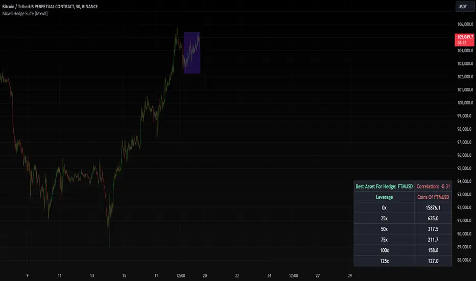
Mxwll Hedge Suite [Mxwll]Hello Traders!
The Mxwll Hedge Suite determines the best asset to hedge against the asset on your chart!
By determining correlation between the asset on your chart and a group of internally listed assets, the Mxwll Hedge Suite determines which asset from the list exhibits the highest negative correlation, and then determines exactly how many coins/shares/contracts of the asset must be bought to achieve a perfect 1:1 hedge!
The image above exemplifies the process!
The purple box on the chart shows the eligible price action used to determine correlation between the asset on my chart (BTCUSDT.P) and the list of cryptocurrencies that can be used as a hedge!
From this price action, the coin determined to have to greatest negative correlation to BTCUSDT.P is FTMUSD.
The image above further outlines the hedge table located in the bottom-right corner of your chart!
The hedge table shows exactly how many coins you’d need to purchase for the hedge asset at various leverages to achieve a perfect 1:1 hedge!
Hedge Suite works on any asset on any timeframe!
And that’s all! A short and sweet script that is hopefully helpful to traders looking to hedge their positions with a negatively correlated asset!
Thank you, Traders!
LETF Leveraged Edge Strategy v1.5Overview
The strategy is based on Stochastics to detect trends and then makes Buys and Sell based on custom entry and exit criteria as described below in the Execution Logic Rules section. It will NOT work with standard Stochastics.
This is not a standard Stochastics implementation. It has been customized and modified, and does not match any widely known Stochastics variations (like Fast, Slow, or Full Stochastics) in its smoothing and iterative calculation process with:
• A unique smoothing mechanism.
• Iterative calculations.
• Additional conditional logic for strategy execution.
This strategy is designed to focus on volatile, liquid leveraged ETFs to capture gains equal to or better than Buy and Hold, and mitigate the risk of trading with a goal of reducing drawdown to a lot less than Buy and Hold. It has had successful backtest performance to varying degrees with TQQQ, SOXL, FNGU, TECL, FAS, UPRO, NAIL and SPXL. Results have not been good on other LETFs that have been backtested.
Performance
In this backtest the Net Profit shows to be $4,561 or 45.61%. Considering the initial order size was $1,000 I have to wonder if the Strategy Tester is calculating this correctly. The Strategy Tester Performance Summary shows the Buy and Hold Return at $61,165 or 611.7%. Based on calculating the price of the last shares sold, less the price paid, times the number of initial shares purchased, my math shows the Buy and Hold Gain at $4,572 or about equal with the strategy performance in this case. The Performance Summary also states the strategy had a Max DD of 3.46% which I believe is incorrect. Based on other backtests I’ve done, I believe the strategy drawdown here was closer to 28.4% and the Buy and Hold Drawdown at 82.7%. I manually calculated the Buy and Hold drawdown.
How it Works
The author provides training and support resource materials for this at his website. The strategy execution logic is driven by these rules:
Execution Logic Rules
Buy the LETF When:
BR #1a) The Daily Fast Line (FL) crosses above the Daily Slow Line (SL) and the FL is between the Low (L*) and High (H*) Range set (often referred to as Oversold and Overbought Lines). This can execute (Buy) any trading day of the week.
BR #1b) Re-Buy the next day after any Stop or Take Profit Sell if the Buy Rule condition is true (FL is above SL), if not, remain in cash and wait for the next Buy Signal.
Sell the LETF When:
SR #1a) The Daily Fast Line (FL) crosses below Daily Slow Line (SL) within the Low (L*) and High (H*) Range (often referred to as Oversold and Overbought Lines). “Crossunder Range Exit” This can execute (Sell) any trading day of the week.
SR #1b) If the (FL) crosses Below the SL above the Exit Level*, wait. Only Sell if the FL drops down below the Exit Level* “Crossunder Level Exit” This can execute (Sell) any trading day of the week.
SR #2a) Sell at the open any day the gap-down price is at or below the 1-Day Stop%*, based on previous day’s closing price (Execute on the day it happens.)
SR #2b) Sell intraday any day the price is at or below the 1-Day Stop %*, based on previous day’s closing price (Execute on the day it happens.)
SR #3a) Sell at the open any day the price is at or below the Trailing Stop %*, based on highest intraday price since Buy date (Execute on the day it happens.)
SR #3b) Sell intraday any day the price is at or below the Trailing Stop%*, based on highest intraday price since Buy date (Execute on the day it happens.)
SR #4) Sell any day when the opening price exceeds, or intraday price meets the Profit Target % price* (Execute on the day it happens.)
SR #5) After each Sell go to Rule BR #1b to determine if a Re-Buy should occur the next day, or stay in cash until next Buy Signal
Settings:
Properties Tab – Initial Capital has been set to $10,000 and order size 10% of Equity, 0.1% commission and 3 Ticks for slippage. Net order size is $1,000
Input Tab:
Stochastic
Timeframe is selected to Daily or Weekly based on preference. Daily has more trades, but on average higher profitability.
Type: Proprietary (best selection for most LETFs, but a few will work better with the Full selection
%k Length 20, %K Smoothing 14, %D Smoothing (many LETFs work better with a specific Stoch setting, often each different) A List of these is provided for your starting point.
Trade Settings
Direction: Longs (This strategy only works on the Long side)
Stop Type: Trailing is recommended, but Fixed is an option.
Stop % (based on user risk tolerance)
PD Stop % (Suggest start at 5%. Based on volatility of LETF and is a stop percentage from prior day’s close. Designed to protect against sudden market volatility. Will need to balance between strategy performance and user risk tolerance)
Profit Target: User preference. (I can help with suggestions based on historical performance)
Entry/Exit Conditions
Enter on Tie: Default Checked – if a Fast line crosses a Slow line for a Buy signal, but doesn’t do so in the range set, this will trigger if it crosses at a tie.
Renter – Default Checked – If stopped out of a position, this tells the strategy to re-buy the position the next day if the conditions are still positive.
Exit Level: This is a exit level for a Fast cross below a Slow line that takes place above the Sell Range, but only happens if the Fast continues down to the level set. These usually don’t happen often, but can have a significant impact on performance. Unfortunately, it’s a trial and error process starting with 90 and working down to see if there’s any positive impact.
Trade Range
Buy Range: Start at typical 20 to 80. Expand the low end down first to check on performance impact. Normally a wide buying range is better for performance.
Sell Range: Start at 20 to 80 and tighten gradually to see performance impact. In some cases a very tight sell range does better. I have worked on our primary LETFs for many months to determine ranges for each that typically produce better results.
External Indicator: Some additional indicators have a positive impact on the strategy performance by increasing P/l, reducing drawdown and reducing the number of trades. This is not always the case and each LETF and time period for the LETF will have a bearing on whether the secondary indicator will help or not. Two that have helped are the MACD Histogram, and the Sloe-Velocity Indicator by Kamleshkumar43. Sometimes a couple of different indicators will have a positive impact, then it’s a personal preference which you pick to use with the strategy.
Since this strategy is focused on a very narrow selection of liquid LETFs, I have a lot of experience experimenting with the settings for the primary ones and can suggest things that will help. Additional training on the rules, working with the settings, and mitigating some of the negative trades during choppy markets is available at the website.
Chart
The strategy can be selected to use either a Daily or Weekly version of stochastic. This is important because the characteristics are different while still generating very good gains and minimal drawdowns. Generally, the daily stochastic will have a greater number of, and certainly more frequent, trades than the weekly stochastic. However, on average the daily version of the stochastic will generates greater profitability.
The Settings tabs have tooltip icons that will assist in inputting values that correspond to the written rules for the strategy, and some include specific rule detail.
Buying
The strategy generates Buy signals with the Fast line crossing over the Slow line within a “Buy Range” which is adjusted based on volatility of the leveraged ETF. This is unique in that a default is set for these entries to occur if the values are tied and doesn’t need to be within the high and low range if that occurs. The trader can select in the strategy for this to occur the same day, if he’s selected a Daily Stochastic timeframe, or at the end of the trading week if he’s selected a Weekly stochastic timeframe. The volatility of a leveraged ETF will sometimes cause a shake-out exit, a trailing stop can be hit, or there can be an exit based on taking a profit. A big part of the timing challenge was how to handle these. The strategy normally (set as a default) will immediately re-buy the next day only if the original buy conditions are still true. This helps capture gains when conditions are still favorable but keeps the trader out when they’re not.
Selling
Exits are handled in several ways. The strategy will exit if there is a fast line cross below a slow line within the “range”. The range is adjusted based on volatility of the leveraged ETF. The exit occurs at the close of the day if the trader has selected to use a Daily stochastic setting. The exit will occur at the end of the trading week if the trader has chosen a weekly stochastic strategy. The trader will set a level based on the instrument and volatility for another exit type. The level will sometimes coincide with the range exit high level but does not need to. If a fast line crosses down through a slow line above the level set, and then comes down to that level, the strategy will exit the position.
Another unique aspect of the strategy is the PD Stop setting. This is short for “Prior Day”, Rather than a normal stop based on the price paid for a position, the PD Stop is based on a percentage drop from the previous day’s closing price. This helps account for the volatility of the leveraged ETF and will cause an exit quickly if there’s a market, or index moving event. This helps capture gains and reduce risk should there be continued pullback.
Exits will also occur based on setting a trailing stop level and profit taking level. These are adjusted based on the leveraged ETFs volatility and historical performance.
Limitations
Choppy, or sideways markets are the most prone to poor performance and potential for being stopped out multiple times. If stopped out two consecutive times, make sure you’re monitoring market health and there are clear signs of a new uptrend such as a 10D and 21D MA in proper alignment and moving up. If you get a Buy signal from the strategy and you’re not confident yet about market and price direction then it’s fine to wait a day, or several days, to enter after the Buy signal when you have greater confidence about market direction. The author can help with a short list of tactical rules developed for these sideways or choppy markets.
This strategy has proven successful backtest results with a very limited set of LETFs as discussed earlier. The author does not know if it will prove successful with any others, or other types of ETFs such as 2X or plain ETFs. A lot more testing needs to be done.
The strategy buys and sells , excluding stops or take profit, at the market close. It can be very challenging to enter an order at market close.
Disclaimer
Please remember that past performance may not be indicative of future results.
Due to various factors, including changing market conditions, the strategy may no longer perform as well as in historical backtesting. This post and the script do not provide any financial advice and are for educational and entertainment purposes only.

Leveraged Chart with Financing, Portfolio DCA & NormalizationLeveraged Investment Simulator with Portfolio DCA & Performance Metrics
Overview:
This indicator helps simulate leveraged investment strategies, incorporating financing costs, Dollar Cost Averaging (DCA), and performance metrics. Ideal for analyzing leveraged growth on price charts or managing portfolios with periodic contributions.
Key Features:
Dual Simulation Modes:
- Chart Mode: Simulate leveraged growth directly on the price chart.
- Portfolio Mode: Track portfolio performance with periodic DCA contributions.
Leverage & Financing Fees:
- Adjustable leverage multiplier.
- Annual financing fees to model borrowing costs.
Dollar Cost Averaging (DCA):
- Set an initial investment and recurring deposit amounts.
- Choose contribution frequency: Monthly, Quarterly, or Yearly.
Performance Metrics:
- Sharpe Ratio: Evaluate risk-adjusted returns.
- Sortino Ratio: Assess downside risk-adjusted performance.
- Maximum Drawdown: Measure the largest decline from a peak.
Customizable Labels:
- Enable or disable specific sections, such as portfolio details and risk metrics.
Inputs:
Symbol selection (default: AAPL).
Data timeframe (e.g., daily, weekly, monthly).
Leverage multiplier and annual financing fees.
Portfolio options: Initial investment, deposit amounts, and frequencies.
Performance analysis options, including a customizable risk-free rate for Sharpe/Sortino ratios.
Toggleable label sections for focused analysis.
How to Use:
Add the indicator to your chart.
Configure the inputs to match your strategy (e.g., leverage factor, financing rates, DCA settings).
Toggle on/off the label sections to display relevant metrics.
Analyze the results:
Chart Mode: Observe leveraged growth on the price chart.
Portfolio Mode: Track portfolio growth, contributions, and performance metrics.
Benefits:
Simulate realistic scenarios with leverage, financing costs, and periodic investments.
Assess performance with advanced metrics like Sharpe and Sortino Ratios.
Identify risk with Maximum Drawdown analysis.
Customize your view for clarity and focus.
This indicator is perfect for traders and investors looking to optimize leveraged strategies or manage portfolios with DCA contributions effectively.

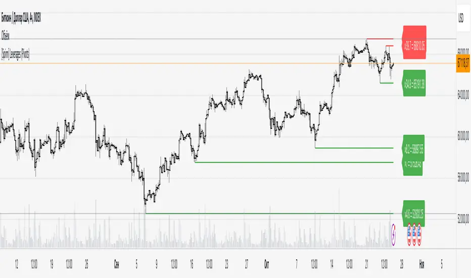
[Spinn] LeveragesThis indicator is designed to visually measure the levels of the position at different leverage values. It acts as a "ruler", the level of levels at which it can cause liquidation, which helps the trader estimate whether it is gradually risky to use this or that leverage.
The indicator works in two modes:
Basic mode:
Levels of prescriptions for standard leverage values (1x, 2x, 5x, etc.), allowing you to quickly assess the risk of consequences when using these coefficients.
Pivots mode:
Levels are built on the basis of local extremes (pivots) on the visible section of the chart, tied to key reversal points.
The pivot is determined by the number of bars to the left and right of it, which is set as a source (the number of bars to the right of each specific roller does not matter).
In this mode, levels will be shown only for the visible part of the chart.
Color marking: green indicates liquidation levels for longs, red - for shorts. Each approach corresponds to a price tag for ease of use.
It is important to note that the indicator uses pure coefficients, without taking into account exchange commissions and other adjustments. Therefore, the calculated levels may not coincide with the actual liquidation levels on the exchanges.
––
Данный индикатор предназначен для визуальной оценки уровней ликвидации позиций при разных значениях плеча. Он выступает в роли «линейки», показывая уровни, на которых может произойти ликвидация, что помогает трейдеру прикинуть, насколько рискованно использовать то или иное плечо.
Индикатор работает в двух режимах:
Режим Basic (базовый):
Уровни привязаны к стандартным значениям плеча (1x, 2x, 5x и т. д.), позволяя быстро оценить риск ликвидации при использовании этих коэффициентов.
Режим Pivots (пивотный):
Уровни строятся на основе локальных экстремумов (пивотов) на видимом участке графика, привязываясь к ключевым точкам разворота.
Пивот определяется по количеству баров слева и справа от него, что задается в настройках (количество баров справа от пивота особой роли не играет).
В этом режиме будут показаны уровни только для видимой части графика.
Цветовая маркировка: зелёным обозначены уровни ликвидаций лонгов, красным — шортов. Каждому уровню соответствует метка с ценой для удобства работы.
Важно отметить, что индикатор использует чистые коэффициенты, без учета комиссий бирж и других поправок. Поэтому рассчитанные уровни могут не совпадать с фактическими уровнями ликвидации на биржах.
LRS-Strategy: 200-EMA Buffer & Long/Short Signals LRS-Strategy: 200-EMA Buffer & Long/Short Signals
This indicator is designed to help traders implement the Leveraged Return Strategy (LRS) using the 200-day Exponential Moving Average (EMA) as a key trend-following signal. The indicator offers clear long and short signals by analyzing the price movements relative to the 200-day EMA, enhanced by customizable buffer zones for increased precision.
Key Features:
200-Day EMA: The main trend indicator. When the price is above the 200-day EMA, the market is considered in an uptrend, and when it is below, it indicates a downtrend.
Customizable Buffer Zones: Users can define a percentage buffer around the 200-day EMA (default is 3%). The upper and lower buffer zones help filter out noise and prevent premature signals.
Precise Long/Short Signals:
Long Signal: Triggered when the price moves from below the lower buffer zone, crosses the 200-day EMA, and then breaks above the upper buffer zone.
Short Signal: Triggered when the price moves from above the upper buffer zone, crosses the 200-day EMA, and then breaks below the lower buffer zone.
Alternating Signals: Ensures that a new signal (long or short) is only generated after the opposite signal has been triggered, preventing multiple signals of the same type without a reversal.
Clear Visual Aids: The indicator displays the 200-day EMA and buffer zones on the chart, along with buy (long) and sell (short) signals. This makes it easy to track trends and time entries/exits.
How to Use:
Long Entry: Look for the price to move below the lower buffer, cross the 200-day EMA from below, and then break out of the upper buffer to confirm a long signal.
Short Entry: Look for the price to move above the upper buffer, cross below the 200-day EMA, and then break below the lower buffer to confirm a short signal.
This indicator is perfect for traders who prefer a structured, trend-following approach, using clear rules to minimize noise and identify meaningful long or short opportunities.

Liquidations [ChartPrime]Liquidations Indicator:
The Liquidations indicator is a powerful tool designed to help traders identify significant liquidation levels in financial markets. By analyzing volume data over a specified lookback period, the indicator highlights potential areas where market participants with high leverage positions may face liquidation, providing valuable insights into market dynamics.
Usage:
Traders can use the Liquidations indicator to:
◈ Identify liquidity grab opportunities: Liquidation levels often attract price action as market participants with leveraged positions face the risk of forced liquidation. Traders can anticipate price movements as the market aims to trigger these stops, potentially leading to rapid price movements or reversals.
◈ Confirm trend strength: A cluster of liquidation levels in the same direction as the prevailing trend may confirm the strength of the trend, while divergences between liquidation levels and price movements may signal potential trend reversals.
Settings:
◈ Previous Value Bars Back: Specifies the number of previous bars used in calculating the liquidation levels.
◈ Show Leverage: Allows users to selectively display liquidation levels for different leverage multiples, including 5x, 10x, 25x, 50x, and 100x.
◈ Liquidation Levels Width: Sets the width of the lines representing liquidation levels on the chart.
◈ Short Liquidations Color: Specifies the color of the lines representing short liquidation levels.
◈ Long Liquidations Color: Specifies the color of the lines representing long liquidation levels.
◈ Bar Color: Sets the color of the background bar when the indicator is active.
Visual Representation:
◈ Liquidation levels are plotted as horizontal lines on the chart, with different colors representing short and long liquidation levels.
◈ Each liquidation level is labeled with the corresponding leverage multiple (e.g., 5x, 10x, etc.).
A dashboard displays the active liquidation levels for each leverage multiple, allowing traders to quickly assess the current market conditions.
◈ Time Window allows users to cut off unnecessary part of the chart and concentrate on a current active part of the chart to make better trading decisions:
Interpretation:
Market participants tend to place stop-loss orders near liquidation levels , creating clusters of pending orders. As price approaches these levels, it may trigger a cascade of stop-loss orders, providing liquidity for market orders and potentially leading to rapid price movements in the opposite direction.
Traders can anticipate price reversals or accelerations as price interacts with liquidation levels, using them as reference points for identifying potential entry or exit opportunities.
Note:
While the Liquidations indicator provides valuable insights into market dynamics, traders should use it in conjunction with other technical analysis tools and risk management strategies to make informed trading decisions.

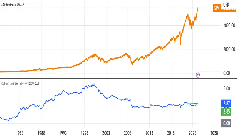
Optimal Leverage IndicatorThe goal of this indicator is to calculate and visualize the optimal leverage and average leverage for a given security based on its historical price data. The optimal leverage is determined by analyzing the relationship between the annualized return and annualized volatility of the security over a specified lookback period.
The methodology can be broken down into the following steps:
Data Input:
The script takes two user inputs: the lookback period and the number of annual trading days.
The lookback period determines the number of historical data points used in the calculations.
The number of annual trading days is used to annualize the return and volatility metrics.
Daily Returns Calculation:
The script retrieves the closing prices of the security on a daily timeframe.
It calculates the daily returns by comparing the current close price with the previous close price.
Mean Return and Volatility Calculation:
The script calculates the mean daily return by taking the simple moving average (SMA) of the daily returns over the specified lookback period.
It also calculates the volatility by taking the standard deviation of the daily returns over the same lookback period.
Annualized Return and Volatility Calculation:
The mean daily return is annualized by compounding it over the number of annual trading days.
The daily volatility is annualized by multiplying it by the square root of the number of annual trading days.
Optimal Leverage Calculation:
The optimal leverage is calculated using the formula: Optimal Leverage = Annualized Return / (Annualized Volatility)^2
This formula assumes that the optimal leverage is proportional to the ratio of the annualized return to the square of the annualized volatility. This is based in this paper: papers.ssrn.com
Average Leverage Calculation:
The script calculates the average leverage by taking the simple moving average (SMA) of the optimal leverage over the specified lookback period.
This provides a smoothed representation of the optimal leverage over time.
The script plots two lines on the chart:
The optimal leverage line (blue) represents the calculated optimal leverage values over time.
The average leverage line (green) represents the average of the optimal leverage values over the specified lookback period.
The main idea behind this methodology is to determine the optimal leverage based on the historical risk-return characteristics of the security. By analyzing the relationship between the annualized return and volatility, the script aims to identify the leverage level that maximizes the return relative to the risk.
The average leverage line provides a smoothed representation of the optimal leverage over time.
AlgoRhythmica - Liquidity StatsThe AlgoRhythmica - Liquidity Stats is a comprehensive trading indicator designed to analyze and plot liquidity data across various time periods. It uses estimated liquidity data and allows traders to select between 6 different scopes to analyze and view that data.
What is liquidity?
Liquidity refers to how quickly and easily an asset can be bought or sold in the market without affecting its price. High liquidity means that there are many buyers and sellers, and transactions can happen rapidly and smoothly.
Liquidity analysis involves examining where and how liquidity is distributed across different price levels.
Price often moves from liquidity zone to liquidity zone, and therefore, having an idea of whether there's more liquidity above or below price give traders an idea of where price might go next.
How does it work?
Internally, the indicator is simulating a complete liquidity map of the chart and cleverly estimates where traders might face losses (liquidations). It does this by looking at the volume of trading in each candle and projecting where, given certain common trading practices like using 10x or 20x leverage, traders are likely to get squeezed out of their positions. These projected squeeze-out points helps in visualizing potential future price movements, as prices often move towards these areas to balance out. But instead of rendering the liquidity on the main chart, which can get cluttered, this data is viewed in a separate panel through a selection of different scopes.
Keep in mind though, this liquidity data here is just an estimation based on general assumptions, it doesn't have access to actual liquidity data.
However, some risk and leverage amounts are more common than others. People like using those even numbers like 10x, 20x leverage or 1% stop loss etc. And that's why the liquidity estimations in this and other liquidity indicators can still be quite accurate.
Special Feature:
A special feature to this indicator is it's unique eye for 'vector candles'—those high-impact candles signaling significant market moves. It tracks these candles over time to see if the market revisits them, a behavior that can indicate major market maker activities and potential price reversal points.
The 6 different plotting scopes:
Liquidity Dominance:
The Liquidity Dominance is the long liquidity minus the short liquidity. When there's more liquidity above price, price tends to go up. There's also a 50 EMA running through it, indicating whether the liquidity dominance is particularly extended.
There is also a setting for normalizing the dominance to an adjustable EMA. Normalizing means that the value of the EMA will then become the zero-value of the dominance. This can be particularly effective in trending markets because it allows traders to see more clearly how the liquidity deviates from it's EMA.
Split Dominance:
This is simply the long and short liquidity plotted separately with a 200 SMA running through. This gives traders a slight more in-depth look at the liquidity. Looking at the difference between long and short liquidity and using the SMA as a reference, traders can more easily spot a trend shift and whether the liquidity types are about to cross each other.
Stochastic LQ:
Instead of using price data, the Stochastic LQ applies the stochastic oscillator formula to liquidity data. It measures the position of the current liquidity level relative to its high-low range over a specified period. By doing so, it aims to provide a clear picture of whether buyers or sellers are dominating the liquidity landscape within the chosen lookback period.
Liquidations:
This will display the amount of volume that was consumed when price wicked or crossed into a liquidity level on that particular bar. There's also a setting to cumulate the liquidations over the selected period. This will show you whether longs or shorts are suffering the most.
Vector Count:
This tool counts the number of unrecovered vector candles. If there are more to the upside, price is likely to go up. The vector count also has a setting for normalizing the count to an EMA. Some older vectors never get recovered and therefore normalizing the count to an EMA can be a more useful way of focusing on more recent vectors.
Total LQ:
By focusing on the total liquidity without differentiating between long and short positions, this tool simplifies the liquidity landscape. High total liquidity can support the sustainability of current trends, as it shows that there is enough market participation to support the price direction.
Additional Features:
Vector Recovery Dots:
A feature to visually identify recovered vector candles, indicating potential market reaction points for strategic entry or exit decisions.
This is used in combination with any of the tools. It will plot dots whenever a vector candle has been recovered. A recovered vector candle while liquidity is extended, could indicate a top or a bottom.
Dynamic Period Selection:
Choose between aggregating the liquidity over a fixed period (Daily, Weekly, Monthly, Yearly etc.) which then stays the same when the user switches timeframe, or choose a dynamic period with a fixed amount of candles which then dynamically shifts when changing time frame. This offers flexibility to look at liquidity over different time frames. Liquidity that falls outside of the selected period is considered gone, as traders eventually close their positions.
Lookback and Sensitivity Adjustment:
Customize the lookback period for volume averages and adjust sensitivity to refine the indicator's responsiveness to volume changes and liquidity calculations.
Leverage Settings:
Input specific leverage amounts to calculate liquidity on. These should be adjusted depending on the chart and timeframe the user is looking at. Decide on up to three different leverage amounts that traders would typically use on the chart and timeframe you're on. The liquidity will then be calculated using that leverage.
Tooltips:
The indicator comes with extensive tooltips for every function, making sure the user understand every part of it.
And as usual, use it together with other market analysis and perhaps a liquidity map of your choice.
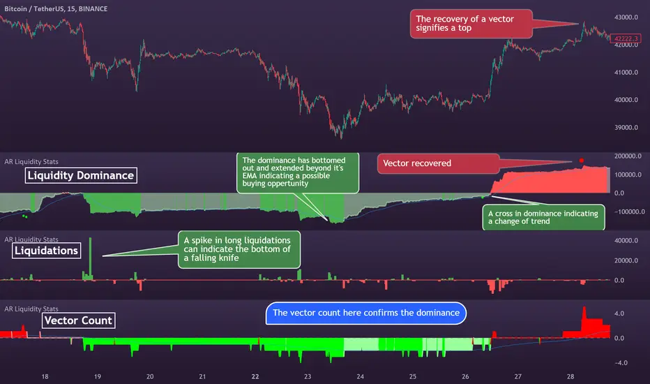
Bitcoin Leverage Sentiment - Strategy [presentTrading]█ Introduction and How it is Different
The "Bitcoin Leverage Sentiment - Strategy " represents a novel approach in the realm of cryptocurrency trading by focusing on sentiment analysis through leveraged positions in Bitcoin. Unlike traditional strategies that primarily rely on price action or technical indicators, this strategy leverages the power of Z-Score analysis to gauge market sentiment by examining the ratio of leveraged long to short positions. By assessing how far the current sentiment deviates from the historical norm, it provides a unique lens to spot potential reversals or continuation in market trends, making it an innovative tool for traders who wish to incorporate market psychology into their trading arsenal.
BTC 4h L/S Performance
local
█ Strategy, How It Works: Detailed Explanation
🔶 Data Collection and Ratio Calculation
Firstly, the strategy acquires data on leveraged long (**`priceLongs`**) and short positions (**`priceShorts`**) for Bitcoin. The primary metric of interest is the ratio of long positions relative to the total of both long and short positions:
BTC Ratio=priceLongs / (priceLongs+priceShorts)
This ratio reflects the prevailing market sentiment, where values closer to 1 indicate a bullish sentiment (dominance of long positions), and values closer to 0 suggest bearish sentiment (prevalence of short positions).
🔶 Z-Score Calculation
The Z-Score is then calculated to standardize the BTC Ratio, allowing for comparison across different time periods. The Z-Score formula is:
Z = (X - μ) / σ
Where:
- X is the current BTC Ratio.
- μ is the mean of the BTC Ratio over a specified period (**`zScoreCalculationPeriod`**).
- σ is the standard deviation of the BTC Ratio over the same period.
The Z-Score helps quantify how far the current sentiment deviates from the historical norm, with high positive values indicating extreme bullish sentiment and high negative values signaling extreme bearish sentiment.
🔶 Signal Generation: Trading signals are derived from the Z-Score as follows:
Long Entry Signal: Occurs when the BTC Ratio Z-Score crosses above the thresholdLongEntry, suggesting bullish sentiment.
- Condition for Long Entry = BTC Ratio Z-Score > thresholdLongEntry
Long Exit/Short Entry Signal: Triggered when the BTC Ratio Z-Score drops below thresholdLongExit for exiting longs or below thresholdShortEntry for entering shorts, indicating a shift to bearish sentiment.
- Condition for Long Exit/Short Entry = BTC Ratio Z-Score < thresholdLongExit or BTC Ratio Z-Score < thresholdShortEntry
Short Exit Signal: Happens when the BTC Ratio Z-Score exceeds the thresholdShortExit, hinting at reducing bearish sentiment and a potential switch to bullish conditions.
- Condition for Short Exit = BTC Ratio Z-Score > thresholdShortExit
🔶Implementation and Visualization: The strategy applies these conditions for trade management, aligning with the selected trade direction. It visualizes the BTC Ratio Z-Score with horizontal lines at entry and exit thresholds, illustrating the current sentiment against historical norms.
█ Trade Direction
The strategy offers flexibility in trade direction, allowing users to choose between long, short, or both, depending on their market outlook and risk tolerance. This adaptability ensures that traders can align the strategy with their individual trading style and market conditions.
█ Usage
To employ this strategy effectively:
1. Customization: Begin by setting the trade direction and adjusting the Z-Score calculation period and entry/exit thresholds to match your trading preferences.
2. Observation: Monitor the Z-Score and its moving average for potential trading signals. Look for crossover events relative to the predefined thresholds to identify entry and exit points.
3. Confirmation: Consider using additional analysis or indicators for signal confirmation, ensuring a comprehensive approach to decision-making.
█ Default Settings
- Trade Direction: Determines if the strategy engages in long, short, or both types of trades, impacting its adaptability to market conditions.
- Timeframe Input: Influences signal frequency and sensitivity, affecting the strategy's responsiveness to market dynamics.
- Z-Score Calculation Period: Affects the strategy’s sensitivity to market changes, with longer periods smoothing data and shorter periods increasing responsiveness.
- Entry and Exit Thresholds: Set the Z-Score levels for initiating or exiting trades, balancing between capturing opportunities and minimizing false signals.
- Impact of Default Settings: Provides a balanced approach to leverage sentiment trading, with adjustments needed to optimize performance across various market conditions.
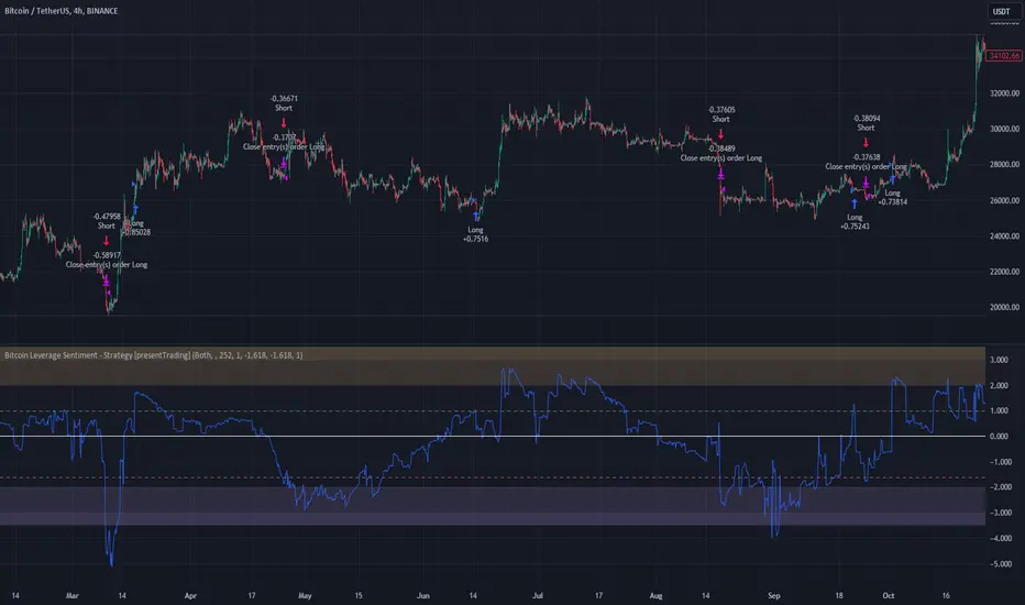
AlgoRhythmica - Liquidity MapThe AlgoRhythmica - Liquidity Map is a complex and performance heavy indicator, attempting to visualize and highlight areas of liquidity on the chart. It paints lines above and below price with different color and opacity based on the volume, and then highlight the areas with the highest cumulative volume.
What is liquidity and a liquidity map?
Liquidity refers to how quickly and easily an asset can be bought or sold in the market without affecting its price. High liquidity means that there are many buyers and sellers, and transactions can happen rapidly and smoothly.
Liquidity analysis involves examining where and how liquidity is distributed across different price levels.
Price often moves from liquidity zone to liquidity zone, and therefore, having an idea of where those zones are can give traders an understanding of potential support and resistance levels and where significant trading activities might occur.
Those looking to fill large buy orders for example would want to do that in liquid sell areas and vice versa. This indicator attempts to estimate the price levels where traders using leverage get liquidated, and therefore creates liquid areas for buying and selling.
In contrast to Bookmaps which chart the orders in the order book where traders want to transact, a liquidity map is charting where traders are 'forced' to transact due to stop-losses or margin calls. To do that, liquidity maps are mostly based on estimations. It could be based on pivot points, common stop-loss amounts, common leverage amounts or a combination of multiple factors.
As of the current version on release, this indicator is only using the leverage input by the user to estimate the liquidity.
How does it work and what makes it unique?
The indicator takes the volume in a candle and saves that volume in a line. Based on the leverage settings it then offsets that line above and below price. Say, a trader using 20x leverage without a stop-loss gets liquidated if price goes roughly 5% in the wrong direction. Therefore, by assuming common leverage amounts or common risk amounts, we can estimate where traders get liquidated or have their stop-losses based on their leverage or amount they are willing to risk.
Now keep in mind, this liquidity map is just estimating based on general assumptions, it doesn't have access to actual liquidity data.
But at the same time, we're not trading single individual traders, but we're trading the market as a whole, and interestingly enough, some risk and leverage amounts are more common than others. People like using those even numbers like 10x, 20x, 1% risk etc. That's why price do often react on the liquidity in liquidity maps such as this one.
So, when a candle is printed, and you are on a smaller timeframe and decided this is just the kind of market for 100x scalpers. You set the leverage to 100x in the settings and the indicator will paint lines above and below price offset by 1%. There are settings for three leverage amounts at the same time, so you might also set it to paint lines at 5% and 10%, just to catch those traders on higher timeframes if price really takes off.
Now let's talk about what makes this indicator really shine and stand out!
Normally, if we just left the indicator doing as above, there would be lines all over the place and very difficult to interpret which areas matter, or we could limit the indicator to only print lines at high volume candles. Now, you do have that option, but that wouldn't pick up areas where low volume trading has cumulated in the same range, such as over a weekend or during market gaps. Where other liquidity indicators out there might miss that liquidity, this indicator has several solutions for it.
The first solution is stacking semi-transparent lines on top of each other. Normally, lines of the same color and transparency wouldn't add and blend together. But this script offers a seamless transition from one color the next, blending those low volume liquidity lines together.
The second solution, and this is what I believe is really unique and powerful, is that this indicator also has the ability highlight certain liquidity. When enabled, it scans through all the lines, cumulate the volume within a specified range around the lines and then compare the cumulated volume range with the ranges around the other lines. New lines created in the range with the highest cumulated volume gets highlighted.
Without this feature you wouldn't necessarily be able to tell which of two strong areas are more liquid. When price later enters that area and crosses those lines, the liquidity there is then considered consumed and lines created in a different range will now begin to highlight.
All of this is of course enhanced, as in the picture above, when multiple copies of the indicator is used together and assigned to only calculate specific parts of the liquidity map, such as longs, shorts or specific leverage amounts.
Oh, and there's also options for assigning which part of the candle should generate the liquidity. Close, Middle Body or Open. The indicator will then assume that the majority of traders are entering their position in that part of the candle.
The offset is calculated from that part of the candle. By using multiple copies of the indicator, you can assign one for each part and that will give you the whole range of the candle. And you might assume more traders go long from the top, so to emphasize that liquidity, you could increase the size or transparency slightly of the lines generated from that part.
How do I use it?
Well, this isn't gonna give you trading signals or anything, but it will visualize the market for you in a new perspective.
Typically, high liquidity areas are often good areas for entry and TP. But always watch how the price reacts in those areas before entering a position. And remember, the liquidity estimation might not always be accurate.
Particularly watch the highlighted areas for long wicks and high volume, indicating that the liquidity was enough to meet the orders and a retrace or reversal could be imminent.
Watch what happens during consolidation, market gaps and weekends. Notice the lack of liquidity and how the market maker creates liquidity by inducing traders to take positions with quick moves that instantly reverses. You might know how that works in theory, but watching it happen real-time with visualized liquidity is very interesting.
While not necessary, and as I've mentioned earlier, dividing the different functions of the indicator on multiple copies will substantially increase it's accuracy and performance!
For example, use one copy of the indicator per leverage level, or one for shorts, one for longs. One that generates from the close, one from the middle etc. creating a much clearer picture of the liquidity like the picture comparison above.
This is what the indicator offers:
When you're estimating liquidity, you want to be able to do it with accuracy and interpretability. That's why the customization options of this indicator has been really important in the development.
Timeframe Options:
It supports a wide range of time periods, from daily to yearly, enabling traders to apply it across various trading strategies, from short-term day trading to long-term investment analysis. Assuming traders are eventually taking their profits, liquidity after the set time period disappears.
Rich Visual Settings:
The indicator comes with multiple preset color themes and a completely customizable option as well. These visual settings are designed to enhance the interpretability of liquidity data, with adjustable transparency and contrast features.
Liquidity Highlighting Function:
This unique feature emphasizes areas with high liquidity concentration. It scans and highlights significant liquidity zones, aiding traders in identifying critical market levels.
Liquidity Profile:
The LQ-Profile extends liquidity lines based on their associated volume, giving traders another way of identifying high liquidity zones.
Adjustable Liquidity Estimation:
Select and adjust leverage amounts based on your particular chart and analysis. Choose what positions and leverage amounts to display liquidity for. You also have the option to determine if wicks consume liquidity or not.
Since wicks indicate that price was rejected from that area, it doesn't necessarily mean all the liquidity in that area was consumed. You could assign an additional copy of the indicator consuming with wicks and another that doesn't. That way, half the liquidity gets consumed and the other half remains until another candle closes in that area. They choices are endless and it's all about your understanding and analysis here.
Multiple Performance Options:
Depending on your particular chart and timeframe, this indicator can be very performance heavy to load. Luckily it has plenty of performance options for limiting the calculations of the indicator.
Tooltips:
As usual, this indicator comes with extensive tooltips for every function, making sure you understand every part of it.
Happy trading!
