Adaptive Regime Z-Score (ARZ)Adaptive Regime Z-Score (ARZ) — Description
Adaptive Regime Z-Score (ARZ) is a regime-weighted, volatility-normalized price deviation histogram.
It measures the distance between price and a slow EMA (market center), normalized by ATR, and amplifies this deviation only when a directional trend regime is confirmed.
The output is displayed as a signed histogram, capped between -100 and +100, with directional regime awareness (bullish or bearish trends).
🔍 What ARZ measures
Normalized price deviation
Distance of price from the EMA center, expressed in ATR units and scaled to a fixed range.
Directional trend regime detection
A trend regime is confirmed only when all three conditions align:
EMA slope has a clear direction
Price is sufficiently far from the EMA (ATR-based distance)
ADX is above its threshold
Regime-weighted deviation
When a trend regime is active, the deviation is scaled by a trend-strength score
When no trend is detected, the output collapses toward zero
📊 How to read the histogram
Green bars → confirmed bullish trend regime
(price extended above EMA, positive deviation)
Red bars → confirmed bearish trend regime
(price extended below EMA, negative deviation)
Near-zero values → no confirmed trend regime
(range / transition state, not highlighted)
There is no separate “ranging” histogram:
absence of bars (or minimal values) implicitly represents non-trending conditions.
🎨 Visual elements
Histogram
Green = bullish trend regime
Red = bearish trend regime
Intensity reflects trend strength × extension
Highlighted only when a directional trend regime is active
Neutral otherwise
Upper / Lower Visual Levels
Reference levels only
Deviation

TTS Orb Orderflow NexusTTS Orb Orderflow Nexus is a comprehensive trading dashboard that combines multiple technical analysis concepts into a single, unified tool. It integrates Opening Range Breakout (ORB) analysis, Anchored VWAP, ES/NQ correlation tracking, volume profile concepts, cumulative volume delta, orderflow patterns, and liquidity detection to help traders identify high-probability setups.
Credits
This indicator was built upon and inspired by Tradeseekers' "Opening Range Breakout and Price Targets" indicator. Full credit to Tradeseekers for the original ORB logic and price target framework that serves as the foundation for this expanded version. This script extends that work by adding correlation analysis, orderflow tools, liquidity detection, and a comprehensive dashboard.
Key Features
15-Minute Opening Range Breakout (ORB)
Automatically identifies and plots the 15-minute opening range (default 8:30-8:45 AM CT)
Displays ORB high, low, mid, and quarter levels
Calculates price targets at 50%, 100%, and 150% extensions
Visual ORB box that extends throughout the trading session
Anchored VWAP with Standard Deviation Bands
VWAP anchored to market open
Configurable 1σ, 2σ, and 3σ standard deviation bands
Identifies extended price conditions and mean reversion zones
ES/NQ Correlation Analysis
Tracks ES1! futures alongside your chart (designed for NQ)
Monitors both instruments' positions relative to their respective ORBs
Detects divergence and convergence between the two markets
Generates setup alerts when one market leads or lags the other
Volume & Orderflow Analysis
Cumulative Volume Delta (CVD) with divergence detection
Buy/sell pressure percentage
Volume ratio compared to 20-period average
High and low volume node identification
Orderflow Pattern Detection
Absorption patterns (high volume with minimal price movement)
Iceberg/hidden order detection
Exhaustion pattern identification
Liquidity Detection
Swing high/low tracking
Liquidity sweep alerts (stop hunts)
Unusual wick detection with configurable thresholds
Rejection candle identification
Candlestick Pattern Recognition
Engulfing patterns
Hammer and shooting star
Doji
Morning and evening star
Dynamic Dashboard
Real-time display of all indicators and their current states
ES/NQ setup recommendations with strength ratings
Confluence scoring system
Position tracking
Fully customizable size and position
Signal Generation
Three signal modes: Aggressive, Conservative, and Ultra-Conservative
Configurable minimum confluence requirements
Automatic long and short entries with exit conditions
Multiple alert conditions for all major events
Recommended Use
This indicator is designed primarily for trading NQ (Nasdaq futures) while monitoring ES (S&P futures) correlation, but can be adapted to other instruments. The ES/NQ correlation setups identify opportunities when one market breaks out or fails while the other lags, providing potential mean-reversion or trend-continuation entries.
Inputs & Customization
Session times and timezone
ORB box colors and styling
VWAP standard deviation multipliers
EMA length
Correlation period
Volume and absorption thresholds
Liquidity sweep parameters
Signal mode and confluence requirements
Dashboard position, size, and colors
🙏 Acknowledgments
Special thanks to Tradeseekers for the original "Opening Range Breakout and Price Targets" indicator. Their work on ORB logic and price target calculations provided the foundation upon which this expanded indicator was built.
⚠️ RISK DISCLAIMER
IMPORTANT: Please read this disclaimer carefully before using this indicator.
This indicator is provided for educational and informational purposes only. It is not intended as, and should not be construed as, financial advice, investment advice, or trading recommendations.
I am not a licensed financial advisor, registered investment advisor, broker, or dealer. I do not provide personalized investment advice or recommendations tailored to your individual circumstances.
Trading futures, options, and other financial instruments involves substantial risk of loss and is not suitable for all investors. You could lose some or all of your initial investment. Only trade with capital you can afford to lose.
Past performance of any trading strategy, indicator, or system is not indicative of future results. No representation is being made that any account will or is likely to achieve profits or losses similar to those discussed or shown.
Before trading:
Understand that all trading involves risk
Never trade with money you cannot afford to lose
Consider consulting with a qualified financial professional
Paper trade and backtest thoroughly before risking real capital
Develop proper risk management and position sizing strategies
By using this indicator, you acknowledge that:
All trading decisions are your own responsibility
You understand and accept the risks involved in trading
The creator of this indicator is not liable for any losses you may incur
No guarantees of profitability are made or implied
Trade responsibly and at your own risk.Claude is AI and can make mistakes. Please double-check responses.

ATR-Normalized VWMA DeviationThis indicator measures how far price deviates from the Volume-Weighted Moving Average ( VWMA ), normalized by market volatility ( ATR ). It identifies significant price reversal points by combining price structure and volatility-adjusted deviation behavior.
The core idea is to use VWMA as a dynamic trend anchor, then measure how far price travels away from it relative to recent volatility . This helps highlight when price has stretched too far and may be due for a reversal or pullback.
How it works:
VWMA deviation is calculated as the difference between price and the VWMA.
That deviation is divided by ATR (Average True Range) to normalize for current volatility.
The script tracks the highest and lowest normalized deviations over the chosen lookback period.
It also tracks price structure (highest/lowest highs/lows) over the same period.
A reversal signal is generated when a historical extreme in deviation aligns with a price structure extreme, and a confirmed reversal candle forms.
You get visual signals and color highlights where these conditions occur.
Settings explained:
Lookback period defines how many bars the script uses to find recent extremes.
ATR length controls how volatility is measured.
VWMA length controls how the volume-weighted moving average is calculated.
Signal filters help refine entries based on price vs deviation behavior.
Display options let you customize how signals and levels appear on the chart.
This indicator is especially useful for spotting potential turning points where price has moved far from VWMA relative to volatility, suggesting possible exhaustion or overextension.
Tips for use:
Combine with broader trend context (higher timeframe support/resistance).
Use with risk management rules (position sizing, stops) — signals are guides, not guaranteed entries.
Adjust lookback and ATR settings based on your trading timeframe and asset volatility.

VWAP Pro [cryptalent]VWAP Pro (Multi-Period + Standard Deviation)
1. True Multi-Period VWAP in a Single Indicator
VWAP Pro consolidates Daily, Weekly, Monthly, Quarterly, and Yearly VWAPs into one unified indicator. This eliminates the need for multiple scripts and allows traders to assess short-, medium-, and long-term value simultaneously on any timeframe.
This design supports:
Multi-timeframe value alignment
Institutional-style reference points
Cleaner charts with fewer indicators
2. Accurate Volume-Weighted Standard Deviation
Unlike generic volatility bands, the standard deviation in VWAP Pro is fully volume-weighted and derived directly from the VWAP calculation. This ensures that dispersion reflects where real trading activity occurred, not just price fluctuation.
Benefits include:
More realistic value boundaries
Improved identification of statistically stretched prices
Reduced noise compared to time-based indicators
3. Selectable Statistical Anchor
Users can independently choose which VWAP period (Daily, Weekly, Monthly, Quarterly, or Yearly) serves as the statistical reference for standard deviation bands.
This allows traders to:
Analyze intraday mean reversion around Daily VWAP
Track swing-level extensions from Weekly or Monthly VWAP
Maintain consistency between strategy horizon and statistical context
4. Current and Previous Period VWAP Visibility
VWAP Pro optionally plots previous period VWAPs alongside current ones. These prior value references often act as:
High-probability reaction levels
Acceptance or rejection zones
Structural support and resistance
This feature provides historical context without clutter, enabling more informed decision-making.
5. Highly Configurable and User-Controlled
Every VWAP and standard deviation component can be toggled independently. Traders can:
Display only relevant periods
Adjust standard deviation multipliers (1σ, 2σ, 3σ)
Customize colors for immediate visual clarity
The indicator adapts easily to different trading styles, from scalping to position trading.
6. Designed for Market Structure and Value Analysis
VWAP Pro is built around value discovery, not prediction. It excels at highlighting:
Fair value zones
Overextended price conditions
Areas where acceptance or rejection is likely to occur
This makes it especially effective for traders focused on market structure, auction behavior, and liquidity-driven price movement.
7. Clean Visualization with Professional Aesthetics
Careful use of transparency, fills, and plotting styles ensures that:
VWAP levels remain clearly visible
Standard deviation zones provide context without dominating the chart
Multiple periods can coexist without visual overload
The result is a professional-grade visual tool suitable for continuous use.
Summary
VWAP Pro (Multi-Period + Standard Deviation) is a comprehensive value-based indicator that combines multi-timeframe VWAPs, volume-weighted statistical bands, and flexible configuration into a single, efficient framework. It is designed for traders who prioritize structure, context, and statistically grounded decision-making over lagging signals or predictive indicators.

Range Deviations PRO | Trade SymmetryRange Deviations PRO — Extended Session Levels
An enhanced version of the original Range Deviations by @joshuuu, retaining the full core logic while adding a key upgrade:
🔹 All session ranges, midlines, and deviation levels now extend into the next trading session, giving seamless multi-session context.
Supports Asia, CBDR, Flout, ONS, and Custom Sessions — with options for half/full standard deviations, equilibrium, and range boxes exactly as in the original.
Extending these levels helps identify:
• Liquidity sweeps
• Trap moves / false breaks
• Daily high/low projections
• Premium–discount behavior across sessions
Ideal for traders using ICT concepts who want clearer continuation of session structure into the next day.
Credit: Original logic by @joshuuu — enhancements by TradeSymmetry.
Disclaimer: Educational use only. Not financial advice.

Tactical Deviation🎯 TACTICAL DEVIATION - Volume-Backed VWAP Deviation Analysis
What Makes This Different?
Unlike basic VWAP indicators, Tactical Deviation combines:
• Multi-timeframe VWAP deviation bands (Daily/Weekly/Monthly)
• Volume spike intelligence - signals only appear with volume confirmation
• Pivot reversal detection at deviation extremes
• Optional multi-VWAP confluence system
• Smart defaults for quality over quantity
This unique combination filters weak setups and identifies high-probability entries at extreme price deviations from fair value.
📊 DEFAULT SETTINGS (Ready to Use)
✅ Daily VWAP with ±2σ deviation bands
✅ Volume spike detection (1.5x average required)
✅ 2σ minimum deviation for signals
❌ Weekly/Monthly VWAPs (enable for multi-timeframe)
❌ Pivot reversal requirement (enable for stronger signals)
❌ Fill zones (optional visual enhancement)
Why: Daily VWAP is most relevant for intraday trading. 2σ bands catch meaningful moves. Volume spikes ensure conviction. Clean chart focuses on what matters.
🚀 HOW TO USE
BASIC USAGE:
• Green triangles (below bars) = Long signals at oversold deviations
• Red triangles (above bars) = Short signals at overbought deviations
SIGNAL QUALITY:
• Normal size, bright colors = Volume spike (best quality)
• Small size, lighter colors = Volume momentum
• Tiny size = No volume confirmation
DEVIATION ZONES:
• ±2σ = Extreme deviation (signals appear here)
• ±1σ to ±2σ = Extended but not extreme
• Within ±1σ = Normal range
TRADING APPROACHES:
Mean Reversion:
→ Enter when price reaches ±2σ with volume spike
→ Target: Return to VWAP or opposite band
→ Stop: Beyond extreme deviation
Trend Continuation:
→ Use bands to identify pullbacks
→ Enter pullback to VWAP in trending market
→ Volume confirms continuation
Reversal Trading:
→ Enable "Require Pivot Reversal" for stronger signals
→ Signals only when deviation + pivot reversal occur
→ Higher probability, fewer signals
⚙️ EXPLORE SETTINGS FOR FULL USE
VWAP SETTINGS:
• Show Weekly/Monthly VWAP = Multi-timeframe context
• Show ±1σ Bands = Normal deviation range
• Show ±3σ Bands = Extreme extremes (rare but powerful)
SIGNAL SETTINGS:
• Min Deviation: 1σ (more signals) | 2σ (default) | 3σ (fewer, extreme only)
• Require Pivot Reversal: OFF (default) | ON (stronger but fewer)
• Volume Spike Threshold: 1.5x (default) | 2.0x+ (major spikes) | 1.2x (more signals)
CONFLUENCE SETTINGS:
• Require Multi-VWAP Confluence: OFF (default) | ON (2+ VWAPs must agree)
• Min VWAPs: 2 (Daily + Weekly/Monthly) | 3 (all must agree)
VISUAL SETTINGS:
• Show Fill Zones = Shaded areas between bands
• Fill Opacity = Transparency adjustment
• Line Widths = Customize thickness
💡 PRO TIPS
1. Start with defaults, then enable features as you learn
2. Volume spike requirement filters weak moves - keep it enabled
3. Enable Weekly/Monthly VWAPs for higher timeframe context
4. Enable confluence for swing trading setups
5. Pivot reversals: ON for reversals, OFF for continuations
6. Check top-right info table for current deviation levels
🎨 VISUAL GUIDE
• Cyan Line = Daily VWAP (fair value)
• Cyan Bands = Daily deviation zones
• Orange Line = Weekly VWAP (if enabled)
• Purple Line = Monthly VWAP (if enabled)
• Green Triangle = Long signal (oversold)
• Red Triangle = Short signal (overbought)
⚠️ IMPORTANT
Educational purposes only. Always use proper risk management. Signals are based on statistical deviation, not guarantees. Volume confirmation improves quality but doesn't guarantee outcomes. Combine with your own analysis.
The unique combination of VWAP deviation analysis, volume profile confirmation, pivot identification, and multi-timeframe confluence in a single clean interface makes Tactical Deviation different from basic VWAP indicators.
Happy Trading! 📈

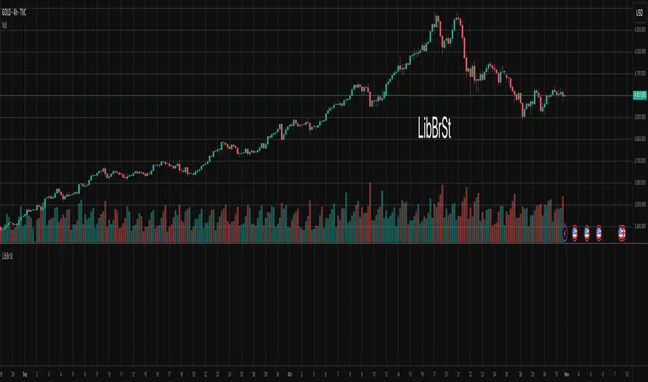
LibBrStLibrary "LibBrSt"
This is a library for quantitative analysis, designed to estimate
the statistical properties of price movements *within* a single
OHLC bar, without requiring access to tick data. It provides a
suite of estimators based on various statistical and econometric
models, allowing for analysis of intra-bar volatility and
price distribution.
Key Capabilities:
1. **Price Distribution Models (`PriceEst`):** Provides a selection
of estimators that model intra-bar price action as a probability
distribution over the range. This allows for the
calculation of the intra-bar mean (`priceMean`) and standard
deviation (`priceStdDev`) in absolute price units. Models include:
- **Symmetric Models:** `uniform`, `triangular`, `arcsine`,
`betaSym`, and `t4Sym` (Student-t with fat tails).
- **Skewed Models:** `betaSkew` and `t4Skew`, which adjust
their shape based on the Open/Close position.
- **Model Assumptions:** The skewed models rely on specific
internal constants. `betaSkew` uses a fixed concentration
parameter (`BETA_SKEW_CONCENTRATION = 4.0`), and `t4Sym`/`t4Skew`
use a heuristic scaling factor (`T4_SHAPE_FACTOR`)
to map the distribution.
2. **Econometric Log-Return Estimators (`LogEst`):** Includes a set of
econometric estimators for calculating the volatility (`logStdDev`)
and drift (`logMean`) of logarithmic returns within a single bar.
These are unit-less measures. Models include:
- **Parkinson (1980):** A High-Low range estimator.
- **Garman-Klass (1980):** An OHLC-based estimator.
- **Rogers-Satchell (1991):** An OHLC estimator that accounts
for non-zero drift.
3. **Distribution Analysis (PDF/CDF):** Provides functions to work
with the Probability Density Function (`pricePdf`) and
Cumulative Distribution Function (`priceCdf`) of the
chosen price model.
- **Note on `priceCdf`:** This function uses analytical (exact)
calculations for the `uniform`, `triangular`, and `arcsine`
models. For all other models (e.g., `betaSkew`, `t4Skew`),
it uses **numerical integration (Simpson's rule)** as
an approximation of the cumulative probability.
4. **Mathematical Functions:** The library's Beta distribution
models (`betaSym`, `betaSkew`) are supported by an internal
implementation of the natural log-gamma function, which is
based on the Lanczos approximation.
---
**DISCLAIMER**
This library is provided "AS IS" and for informational and
educational purposes only. It does not constitute financial,
investment, or trading advice.
The author assumes no liability for any errors, inaccuracies,
or omissions in the code. Using this library to build
trading indicators or strategies is entirely at your own risk.
As a developer using this library, you are solely responsible
for the rigorous testing, validation, and performance of any
scripts you create based on these functions. The author shall
not be held liable for any financial losses incurred directly
or indirectly from the use of this library or any scripts
derived from it.
priceStdDev(estimator, offset)
Estimates **σ̂** (standard deviation) *in price units* for the current
bar, according to the chosen `PriceEst` distribution assumption.
Parameters:
estimator (series PriceEst) : series PriceEst Distribution assumption (see enum).
offset (int) : series int To offset the calculated bar
Returns: series float σ̂ ≥ 0 ; `na` if undefined (e.g. zero range).
priceMean(estimator, offset)
Estimates **μ̂** (mean price) for the chosen `PriceEst` within the
current bar.
Parameters:
estimator (series PriceEst) : series PriceEst Distribution assumption (see enum).
offset (int) : series int To offset the calculated bar
Returns: series float μ̂ in price units.
pricePdf(estimator, price, offset)
Probability-density under the chosen `PriceEst` model.
**Returns 0** when `p` is outside the current bar’s .
Parameters:
estimator (series PriceEst) : series PriceEst Distribution assumption (see enum).
price (float) : series float Price level to evaluate.
offset (int) : series int To offset the calculated bar
Returns: series float Density value.
priceCdf(estimator, upper, lower, steps, offset)
Cumulative probability **between** `upper` and `lower` under
the chosen `PriceEst` model. Outside-bar regions contribute zero.
Uses a fast, analytical calculation for Uniform, Triangular, and
Arcsine distributions, and defaults to numerical integration
(Simpson's rule) for more complex models.
Parameters:
estimator (series PriceEst) : series PriceEst Distribution assumption (see enum).
upper (float) : series float Upper Integration Boundary.
lower (float) : series float Lower Integration Boundary.
steps (int) : series int # of sub-intervals for numerical integration (if used).
offset (int) : series int To offset the calculated bar.
Returns: series float Probability mass ∈ .
logStdDev(estimator, offset)
Estimates **σ̂** (standard deviation) of *log-returns* for the current bar.
Parameters:
estimator (series LogEst) : series LogEst Distribution assumption (see enum).
offset (int) : series int To offset the calculated bar
Returns: series float σ̂ (unit-less); `na` if undefined.
logMean(estimator, offset)
Estimates μ̂ (mean log-return / drift) for the chosen `LogEst`.
The returned value is consistent with the assumptions of the
selected volatility estimator.
Parameters:
estimator (series LogEst) : series LogEst Distribution assumption (see enum).
offset (int) : series int To offset the calculated bar
Returns: series float μ̂ (unit-less log-return).
Matrix bands by JaeheeMatrix Bands — multi-sigma EMA bands for price dispersion context (no signals)
📌 What it is
Matrix Bands draws an EMA-based central line with multiple standard-deviation envelopes at ±1σ, ±1.618σ, ±2σ, ±2.618σ, ±3σ.
Thin core lines show the precise band levels, while subtle outer “glow” lines improve readability without obscuring candles.
📌 How it works (concept)
Basis: EMA of the selected source (default: close)
Dispersion: Rolling sample standard deviation over the same length
Bands: Basis ± k·σ for k ∈ {1, 1.618, 2, 2.618, 3}
This is not a strategy and does not generate trade signals.
It provides price dispersion context only.
📌 Why these levels together (justification of the combination)
Using multiple σ layers reveals graduated risk zones in one view:
±1σ: routine fluctuation
±1.618σ & ±2σ: extended but still common excursions
±2.618σ & ±3σ: statistically rare extremes, where mean-reversion risk or trend acceleration risk increases
Combining these specific multipliers allows traders to judge positioning vs. volatility instantly, without switching between separate indicators or re-configuring a single band.
📌 How it differs from classic Bollinger Bands
Unlike classic Bollinger Bands, which typically use an SMA basis and only ±2σ envelopes,
Matrix Bands uses an EMA basis for faster trend responsiveness and plots five sigma levels (±1, ±1.618, ±2, ±2.618, ±3).
This design allows traders to visualize market dispersion across multiple statistical thresholds simultaneously, making it more versatile for both trend-following and mean-reversion contexts.
📌 How to read it (context, not signals)
Mean-reversion context: Moves beyond ±2σ may indicate stretched conditions; wait for your own confirmation signals before acting
Trend context: In strong trends, price can “ride” the outer bands; sustained closes near +2σ~+3σ (uptrend) or −2σ~−3σ (downtrend) suggest persistent momentum
Regime observation: Band width expands in high volatility and contracts in quiet regimes; adjust stops and sizing accordingly
📌 Inputs
BB Length: lookback period for EMA and σ (default: 20)
Source: price source for calculations
📌 Design notes
Thin inner lines = exact levels
Soft outer lines = readability “glow” only; no effect on calculations
Overlay display keeps the chart uncluttered
📌 Limitations & good practice
No entry/exit logic; use with your own strategy rules
Volatility interpretation varies by timeframe
Past patterns do not guarantee future outcomes; risk management is essential
📌 Defaults & scope
Works on any symbol with OHLCV
No alerts, no strategy results, no performance claims

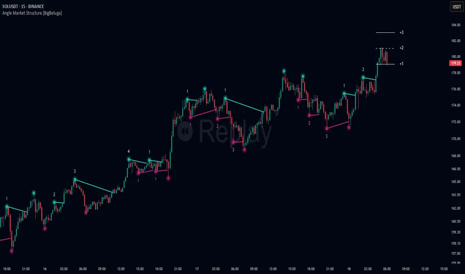
Angle Market Structure [BigBeluga]🔵 OVERVIEW
Angle Market Structure is a smart pivot-based tool that dynamically adapts to price action by accelerating breakout and breakdown detection. It draws market structure levels based on pivot highs/lows and gradually adjusts those levels closer to price using an angle threshold. Upon breakout, the indicator projects deviation zones with labeled levels (+1, +2, +3 or −1, −2, −3) to track price extension beyond structure.
🔵 CONCEPTS
Adaptive Market Structure: Uses pivots to define structure levels, which dynamically angle closer to price over time to capture breakouts sooner.
Breakout Acceleration: Pivot high levels decrease and pivot low levels increase each bar using a user-defined angle (based on ATR), improving reactivity.
Deviation Zones: Once a breakout or breakdown occurs, 3 deviation levels are projected to show how far price extends beyond the breakout point.
Count Labels: Each successful structure break is numbered sequentially, giving traders insight into momentum and trend persistence.
Visual Clarity: The script uses colored pivot points, trend lines, and extension labels for easy structural interpretation.
🔵 FEATURES
Calculates pivot highs and lows using a customizable length.
Applies an angle modifier (ATR-based) to gradually pull levels closer to price.
Plots breakout and breakdown lines in distinct colors with automatic extension.
Shows deviation zones (+1, +2, +3 or −1, −2, −3) after breakout with customizable size.
Color-coded labels for trend break count (bullish or bearish).
Dynamic label sizing and theme-aware colors.
Smart label positioning to avoid chart clutter.
Built-in limit for deviation zones to maintain clarity and performance.
🔵 HOW TO USE
Use pivot-based market structure to identify breakout and breakdown zones.
Watch for crossover (up) or crossunder (down) events as trend continuation or reversal signals.
Observe +1/+2/+3 or -1/-2/-3 levels for overextension opportunities or trailing stop ideas.
Use breakout count as a proxy for trend strength—multiple counts suggest momentum.
Combine with volume or order flow tools for higher confidence entries at breakout points.
Adjust the angle setting to fine-tune sensitivity based on market volatility.
🔵 CONCLUSION
Angle Market Structure enhances traditional pivot-based analysis by introducing breakout acceleration and structured deviation tracking. It’s a powerful tool for traders seeking a cleaner, faster read on market structure and momentum strength—especially during impulsive price moves or structural transitions.
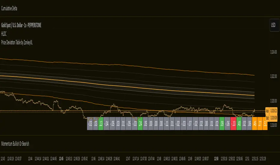
Price Deviation Table by ZonkeyXLProvides a 30 column table showing price deviation per bar close, highlighting larger deviations in red (downside) or green (upside).
Deviations that get highlighted in red/green are calculated to be 2x the amount of price movement in the previous candle, but can be customised to check any deviation size you want in the options panel.
Can be used on any timeframe but you need to specify the number of bars per table column to make it accurate to what you want.
Examples:
If used on the 1 second time frame you could specify bars to 1 and then each column value will check the price as at close on the most recent second for deviations against the close of price on the second prior, showing comparisons up to 30 seconds.
If on the 1 minute time-frame you could specify bars to 2 and then each column value would show deviations from most recent price close to 2 minutes ago, making all 30 columns show deviations for up to an hour.
At the end of the column are 3 orange coloured columns. The first one compares price to 10 bars ago. The second compares current price to 20 bars ago. The 3rd compares current price to 30 bars ago.
In our example on the 1 second above, this would mean deviation is calculated by comparing most recent close to 10 seconds ago, then to 20 seconds ago, and then to 30 seconds ago. The final 3 columns do not highlight red or green, so you can differentiate them properly from the main deviation columns at all times.
Note that the table is rolling - so once it is populated for the first time, only the final column will update while the prior values will shift one column to the left.
Dynamic Gap Probability ToolDynamic Gap Probability Tool measures the percentage gap between price and a chosen moving average, then analyzes your chart history to estimate the likelihood of the next candle moving up or down. It dynamically adjusts its sample size to ensure statistical robustness while focusing on the exact deviation level.
Originality and Value:
• Combines gap-based analysis with dynamic sample aggregation to balance precision and reliability.
• Automatically extends the sample when exact matches are scarce, avoiding misleading signals on rare extreme moves.
• Provides real “next-candle” probabilities based on historical occurrences rather than fixed thresholds or untested heuristics.
• Adds value by giving traders an evidence-based edge: you see how similar past deviations actually played out.
How It Works:
1. Calculate gap = (close – moving average) / moving average * 100.
2. Round the absolute gap to nearest percent (X%).
3. Count historical bars where gap ≥ X% above or ≤ –X% below.
4. If exact X% count is below the minimum occurrences threshold, include gaps at X+1%, X+2%, etc., until threshold is reached.
5. Compute “next-candle” green vs. red probabilities from the aggregated sample.
6. Display current gap, sample size, green probability, and red probability in a table.
Inputs:
• Moving Average Type (SMA, EMA, WMA, VWMA, HMA, SMMA, TMA)
• Moving Average Period (default 200)
• Minimum Occurrences Threshold (default 50)
• Table position and styling options
Examples:
• If price is 3% above the 200-period SMA and 120 occurrences ≥3% are found, with 84 green next candles (70%) and 36 red (30%), the script displays “3% | 120 | 70% green | 30% red.”
• If price is 8% below the SMA but only 20 exact matches exist, the script will include 9% and 10% gaps until it reaches 50 samples, then calculate probabilities from that broader set.
Why It’s Useful:
• Mean-reversion traders see green-probability signals at extreme overbought or oversold levels.
• Trend-followers identify continuation likelihood when red probability is high.
• Risk managers gauge reliability by inspecting sample size before acting on any signal.
Limitations:
• Historical probabilities do not guarantee future performance.
• Results depend on timeframe and symbol, backtest with your data before trading.
• Use realistic slippage and commission when overlaying on strategy scripts.

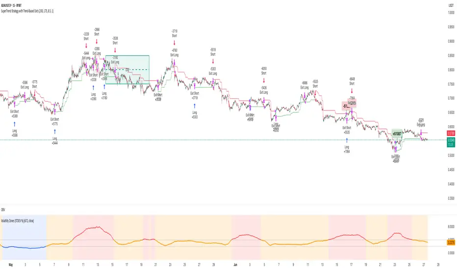
Volatility Zones (STDEV %)This indicator displays the relative volatility of an asset as a percentage, based on the standard deviation of price over a custom length.
🔍 Key features:
• Uses standard deviation (%) to reflect recent price volatility
• Classifies volatility into three zones:
Low volatility (≤2%) — highlighted in blue
Medium volatility (2–4%) — highlighted in orange
High volatility (>4%) — highlighted in red
• Supports visual background shading and colored line output
• Works on any timeframe and asset
📊 This tool is useful for identifying low-risk entry zones, periods of expansion or contraction in price behavior, and dynamic market regime changes.
You can adjust the STDEV length to suit your strategy or timeframe. Best used in combination with your entry logic or trend filters.
Z Score Overlay [BigBeluga]🔵 OVERVIEW
A clean and effective Z-score overlay that visually tracks how far price deviates from its moving average. By standardizing price movements, this tool helps traders understand when price is statistically extended or compressed—up to ±4 standard deviations. The built-in scale and real-time bin markers offer immediate context on where price stands in relation to its recent mean.
🔵 CONCEPTS
Z Score Calculation:
Z = (Close − SMA) ÷ Standard Deviation
This formula shows how many standard deviations the current price is from its mean.
Statistical Extremes:
• Z > +2 or Z < −2 suggests statistically significant deviation.
• Z near 0 implies price is close to its average.
Standardization of Price Behavior: Makes it easier to compare volatility and overextension across timeframes and assets.
🔵 FEATURES
Colored Z Line: Gradient coloring based on how far price deviates—
• Red = oversold (−4),
• Green = overbought (+4),
• Yellow = neutral (~0).
Deviation Scale Bar: A vertical scale from −4 to +4 standard deviations plotted to the right of price.
Active Z Score Bin: Highlights the current Z-score bin with a “◀” arrow
Context Labels: Clear numeric labels for each Z-level from −4 to +4 along the side.
Live Value Display: Shows exact Z-score on the active level.
Non-intrusive Overlay: Can be applied directly to price chart without changing scaling behavior.
🔵 HOW TO USE
Identify overbought/oversold areas based on +2 / −2 thresholds.
Spot potential mean reversion trades when Z returns from extreme levels.
Confirm strong trends when price remains consistently outside ±2.
Use in multi-timeframe setups to compare strength across contexts.
🔵 CONCLUSION
Z Score Overlay transforms raw price action into a normalized statistical view, allowing traders to easily assess deviation strength and mean-reversion potential. The intuitive scale and color-coded display make it ideal for traders seeking objective, volatility-aware entries and exits.

Head Hunter HHHead Hunter HH - Advanced Market Structure & Volume Analysis Indicator
This indicator combines volume analysis, price action, and VWAP to identify high-probability trading opportunities across multiple timeframes.
Key Features:
• Smart Volume Analysis: Detects institutional volume patterns using dynamic thresholds
• VWAP-Based Market Structure: Multiple standard deviation bands for precision entry/exit
• Daily Level Integration: Previous day's high, low, close, and current day's open
• Advanced Signal Classification: Regular, Super Strong, and Scalp signals
Signal Types:
1. Regular Signals (White/Purple Triangles)
• Volume-confirmed reversals
• Institutional price levels
• Technical momentum alignment
2. Super Strong Signals (Green/Red Diamonds)
• High-volume breakouts
• Strong momentum confirmation
• Multiple timeframe alignment
3. Scalp Signals (Green/Magenta Circles)
• Quick reversal opportunities
• VWAP deviation analysis
• Volume surge confirmation
Visual Components:
• VWAP with Standard Deviation Bands
• 50 MA (optional)
• Daily Reference Levels
• Color-coded signals based on strength
• Bar color changes on confirmed signals
Best Practices:
• Most effective on higher timeframes (1H+)
• Use with major pairs/instruments
• Combine signals with support/resistance
• Monitor volume confirmation
• Wait for candle close confirmation
This indicator helps identify institutional order flow and high-probability reversal zones by analyzing volume patterns, price action, and market structure, providing traders with multiple confirmation layers before entry.
Note: Results may vary based on market conditions and timeframe selection. Always use proper risk management.

Directional Deviation Index (DDI)Directional Deviation Index (DDI) is a streamlined, adaptive indicator for analyzing market cycles, detecting trend direction, and gauging momentum. By measuring how far price deviates from a smoothed average, the DDI adapts dynamically to both bullish and bearish conditions.
Key Features:
Unified Smoothing: Choose SMA or EMA for consistent, predictable signals.
Log Scale: Focus on percentage-based moves—ideal for volatile or higher-priced assets.
Adaptive Trend Levels: Auto-adjust uptrend/downtrend thresholds based on market volatility.
Momentum Visualization: Transparent color fills (green for uptrends, red for downtrends) that intensify with stronger deviations.
Customizable Sensitivity: Fine-tune uptrend and downtrend settings to suit any trading style.
Simple Alerts & Status Line: Get notified on key crossovers and track real-time price without chart clutter.
Comparison to Similar Indicators:
Bollinger Bands: Both use deviations from a moving average, but the DDI emphasizes directional momentum and adaptive threshold levels rather than fixed bands.
RSI/Stochastics: While these oscillators focus on overbought or oversold conditions, the DDI tracks how far price strays from its average, giving a clearer picture of trend strength.
MACD: MACD is built on EMA crossovers, whereas the DDI highlights deviations from a mean and adapts more directly to volatility changes.
Use the DDI to identify trend strength, spot potential reversals, and monitor evolving market conditions across stocks, crypto, forex, and beyond. It’s a versatile yet concise tool for traders seeking faster, more confident decisions.

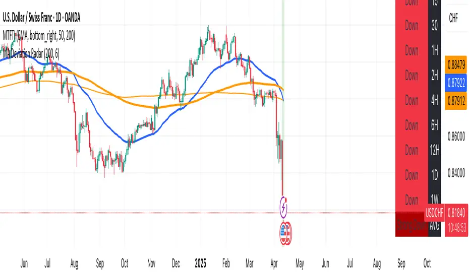
MA Deviation// -----------------------------------------------------------------------------
// MA Deviation Marking & Alert (MA Divergence)
// -----------------------------------------------------------------------------
// Short Title: MA Deviation Radar
// Author: zhipeng luo
// Version: 1.0
// Date: 2025-04-11
// -----------------------------------------------------------------------------
// Overview:
// This indicator identifies and highlights price bars where the closing price
// deviates significantly from its Simple Moving Average (SMA) by a user-defined
// percentage. It visually marks these bars on the chart and provides
// configurable alert conditions for threshold breaches.
//
// How it Works:
// 1. Calculates the Simple Moving Average (SMA) based on the 'MA Period' input.
// 2. Computes the percentage deviation of the closing price from the SMA value.
// Formula: `((Close - SMA) / SMA) * 100`
// 3. Compares the calculated deviation percentage against the positive and
// negative 'Threshold (%)' input values.
// 4. Marks the background of the price bars when a threshold is exceeded:
// - Red Background: Price deviation is greater than the positive threshold.
// - Green Background: Price deviation is less than the negative threshold.
// 5. Includes an optional, non-visible plot of the MA line itself.
// 6. Offers three distinct alert conditions for automation and notifications.
//
// Features:
// - Customizable Simple Moving Average period.
// - Adjustable deviation threshold percentage.
// - Clear visual signals using background colors on the main chart.
// - Built-in Alert Conditions:
// - MA Positive Deviation Alert (Triggers when price > MA + Threshold %)
// - MA Negative Deviation Alert (Triggers when price < MA - Threshold %)
// - MA Deviation Alert - Any (Triggers on either positive or negative breach)
//
// How to Use:
// - Identify Potential Extremes: Useful for spotting potential overbought (large
// positive deviation) or oversold (large negative deviation) conditions
// which might precede price corrections or mean reversion.
// - Gauge Trend Extension: Extreme deviations can sometimes indicate that a
// trend is overextended and might be due for a pause or reversal.
// - Parameter Tuning: Adjust the 'MA Period' and '(Threshold %)' settings to
// suit the specific asset, timeframe, and volatility characteristics you
// are analyzing. Lower thresholds yield more signals; higher thresholds
// focus on more significant deviations.
// - Alerts: Set up alerts via the TradingView alert menu using the provided
// conditions ("MA Positive Deviation Alert", "MA Negative Deviation Alert",
// "MA Deviation Alert - Any") to get notified of potential setups.
//
// Parameters:
// - MA Period (Default: 200): The lookback period for the SMA calculation.
// - (Threshold %) (Default: 7.0): The percentage deviation (positive and
// negative) from the MA required to trigger a background signal and alert.
//
// Alerts & Important Note:
// Three alert conditions corresponding to the signals are available:
// 1. "MA Positive Deviation Alert"
// 2. "MA Negative Deviation Alert"
// 3. "MA Deviation Alert - Any"
//
// ***Please Note:*** The value shown after "( {{plot_0}}%)" or
// "( {{plot_0}}%)" in the default alert message refers to the
// **Moving Average value** (`plot_0`), not the actual deviation percentage.
// The alert *triggers correctly* based on the deviation percentage crossing
// the threshold, but the number displayed by the `{{plot_0}}` placeholder
// in the message is the MA's value at that time due to the script's
// internal plot order.
//
// Disclaimer: This indicator is provided for informational and analytical
// purposes only. It does not constitute financial advice or a recommendation
// to buy or sell any asset. Always conduct your own research and use proper
// risk management. Trading involves significant risk.
// -----------------------------------------------------------------------------
ZVOL — Z-Score Volume Heatmapⓩ ZVOL transforms raw volume into a statistically calibrated heatmap using Z-score thresholds. Unlike classic volume indicators that rely on fixed MA comparisons, ZVOL calculates how many standard deviations each volume bar deviates from its mean. This makes the reading adaptive across timeframes and assets, in order to distinguish meaningful crowd behavior from random volatility.
📊 The core display is a five-zone histogram, each encoded by color and statistical depth. Optional background shading mirrors these zones across the entire pane, revealing subtle compression or structural rhythm shifts across time. By grounding the volume reading in volatility-adjusted context, ZVOL inhibits impulsive trading tactics by compelling the structure, not the sentiment, to dictate the signal.
🥵 Heatmap Coloration:
🌚 Suppressed volume — congestion, coiling phases
🩱 Stable flow — early trend or resting volume
🏀 High activity — emerging pressure
💔 Extreme — possible climax or institutional print
🎗️ A dynamic Fibonacci-based 21:34-period EMA ribbon overlays the histogram. The fill area inverts color on crossover, providing a real-time read on tempo, expansion, or divergence between price structure and crowd effort.
💡 LTF Usage Suggestions:
• Confirm breakout legs when orange or red zones align with range exits
• Fade overextended moves when red bars appear into resistance
• Watch for rising EMAs and orange volume to front-run impulsive moves
• Combine with volatility suppression (e.g. ATR) to catch compression → expansion transitions
🥂 Ideal Pairings:
• OBVX Conviction Bias — to confirm directional intent behind volume shifts
• SUPeR TReND 2.718 — for directional filters
• ATR Turbulence Ribbon — to detect compression phases
👥 The OBVX Conviction Bias adds a second dimension to ZVOL by revealing whether crowd effort is aligning with price direction or diverging beneath the surface. While ZVOL identifies statistical anomalies in raw volume, OBVX tracks directional commitment using cumulative volume and moving average cross logic. Use them together to spot fake-outs, anticipate structure-confirmed breakouts, or time pullbacks with volume-based conviction.
🔬 ZVOL isn’t just a volume filter — it’s a structural lens. It reveals when crowd effort is meaningful, when it's fading, and when something is about to shift. Designed for structure-aware traders who care about context, not noise.

LinearRegressionLibrary "LinearRegression"
Calculates a variety of linear regression and deviation types, with optional emphasis weighting. Additionally, multiple of slope and Pearson’s R calculations.
calcSlope(_src, _len, _condition)
Calculates the slope of a linear regression over the specified length.
Parameters:
_src (float) : (float) The source data.
_len (int) : (int) The length of the lookback period for the linear regression.
_condition (bool) : (bool) Flag to enable calculation. Set to true to calculate on every bar; otherwise, set to barstate.islast for efficiency.
Returns: (float) The slope of the linear regression.
calcReg(_src, _len, _condition)
Calculates a basic linear regression, returning y1, y2, slope, and average.
Parameters:
_src (float) : (float) The source data series.
_len (int) : (int) The length of the lookback period.
_condition (bool) : (bool) Flag to enable calculation (true = calculate).
Returns: (float ) An array of 4 values: .
calcRegStandard(_src, _len, _emphasis, _condition)
Calculates an Standard linear regression with optional emphasis.
Parameters:
_src (float) : (series float) The source data series.
_len (int) : (int) The length of the lookback period.
_emphasis (float) : (float) The emphasis factor: 0 for equal weight; >0 emphasizes recent bars; <0 emphasizes older bars.
_condition (bool) : (bool) Flag to enable calculation (true = calculate).
Returns: (float ) .
calcRegRidge(_src, _len, lambda, _emphasis, _condition)
Calculates a ridge regression with optional emphasis.
Parameters:
_src (float) : (float) The source data series.
_len (int) : (int) The length of the lookback period.
lambda (float) : (float) The ridge regularization parameter.
_emphasis (float) : (float) The emphasis factor: 0 for equal weight; >0 emphasizes recent bars; <0 emphasizes older bars.
_condition (bool) : (bool) Flag to enable calculation (true = calculate).
Returns: (float ) .
calcRegLasso(_src, _len, lambda, _emphasis, _condition)
Calculates a Lasso regression with optional emphasis.
Parameters:
_src (float) : (float) The source data series.
_len (int) : (int) The length of the lookback period.
lambda (float) : (float) The Lasso regularization parameter.
_emphasis (float) : (float) The emphasis factor: 0 for equal weight; >0 emphasizes recent bars; <0 emphasizes older bars.
_condition (bool) : (bool) Flag to enable calculation (true = calculate).
Returns: (float ) .
calcElasticNetLinReg(_src, _len, lambda1, lambda2, _emphasis, _condition)
Calculates an Elastic Net regression with optional emphasis.
Parameters:
_src (float) : (float) The source data series.
_len (int) : (int) The length of the lookback period.
lambda1 (float) : (float) L1 regularization parameter (Lasso).
lambda2 (float) : (float) L2 regularization parameter (Ridge).
_emphasis (float) : (float) Emphasis factor: 0 for equal weight; >0 emphasizes recent bars; <0 emphasizes older bars.
_condition (bool) : (bool) Flag to enable calculation (true = calculate).
Returns: (float ) .
calcRegHuber(_src, _len, delta, iterations, _emphasis, _condition)
Calculates a Huber regression using Iteratively Reweighted Least Squares (IRLS).
Parameters:
_src (float) : (float) The source data series.
_len (int) : (int) The length of the lookback period.
delta (float) : (float) Huber threshold parameter.
iterations (int) : (int) Number of IRLS iterations.
_emphasis (float) : (float) Emphasis factor: 0 for equal weight; >0 emphasizes recent bars; <0 emphasizes older bars.
_condition (bool) : (bool) Flag to enable calculation (true = calculate).
Returns: (float ) .
calcRegLAD(_src, _len, iterations, _emphasis, _condition)
Calculates a Least Absolute Deviations (LAD) regression via IRLS.
Parameters:
_src (float) : (float) The source data series.
_len (int) : (int) The length of the lookback period.
iterations (int) : (int) Number of IRLS iterations for LAD.
_emphasis (float) : (float) Emphasis factor: 0 for equal weight; >0 emphasizes recent bars; <0 emphasizes older bars.
_condition (bool) : (bool) Flag to enable calculation (true = calculate).
Returns: (float ) .
calcRegBayesian(_src, _len, priorMean, priorSpan, sigma, _emphasis, _condition)
Calculates a Bayesian linear regression with optional emphasis.
Parameters:
_src (float) : (float) The source data series.
_len (int) : (int) The length of the lookback period.
priorMean (float) : (float) The prior mean for the slope.
priorSpan (float) : (float) The prior variance (or span) for the slope.
sigma (float) : (float) The assumed standard deviation of residuals.
_emphasis (float) : (float) Emphasis factor: 0 for equal weight; >0 emphasizes recent bars; <0 emphasizes older bars.
_condition (bool) : (bool) Flag to enable calculation (true = calculate).
Returns: (float ) .
calcRFromLinReg(_src, _len, _slope, _average, _y1, _condition)
Calculates the Pearson correlation coefficient (R) based on linear regression parameters.
Parameters:
_src (float) : (float) The source data.
_len (int) : (int) The length of the lookback period.
_slope (float) : (float) The slope of the linear regression.
_average (float) : (float) The average value of the source data series.
_y1 (float) : (float) The starting point (y-intercept of the oldest bar) for the linear regression.
_condition (bool) : (bool) Flag to enable calculation. Set to true to calculate on every bar; otherwise, set to barstate.islast for efficiency.
Returns: (float) The Pearson correlation coefficient (R) adjusted for the direction of the slope.
calcRFromSource(_src, _len, _condition)
Calculates the correlation coefficient (R) using a specified length and source data.
Parameters:
_src (float) : (float) The source data.
_len (int) : (int) The length of the lookback period.
_condition (bool) : (bool) Flag to enable calculation. Set to true to calculate on every bar; otherwise, set to barstate.islast for efficiency.
Returns: (float) The correlation coefficient (R).
calcSlopeLengthZero(_src, _len, _minLen, _step, _condition)
Identifies the length at which the slope is flattest (closest to zero).
Parameters:
_src (float) : (float) The source data.
_len (int) : (int) The maximum lookback length to consider (minimum of 2).
_minLen (int) : (int) The minimum length to start from (cannot exceed the max length).
_step (int) : (int) The increment step for lengths.
_condition (bool) : (bool) Flag to enable calculation. Set to true to calculate on every bar; otherwise, set to barstate.islast.
Returns: (int) The length at which the slope is flattest.
calcSlopeLengthHighest(_src, _len, _minLen, _step, _condition)
Identifies the length at which the slope is highest.
Parameters:
_src (float) : (float) The source data.
_len (int) : (int) The maximum lookback length (minimum of 2).
_minLen (int) : (int) The minimum length to start from.
_step (int) : (int) The step for incrementing lengths.
_condition (bool) : (bool) Flag to enable calculation. Set to true to calculate on every bar; otherwise, set to barstate.islast.
Returns: (int) The length at which the slope is highest.
calcSlopeLengthLowest(_src, _len, _minLen, _step, _condition)
Identifies the length at which the slope is lowest.
Parameters:
_src (float) : (float) The source data.
_len (int) : (int) The maximum lookback length (minimum of 2).
_minLen (int) : (int) The minimum length to start from.
_step (int) : (int) The step for incrementing lengths.
_condition (bool) : (bool) Flag to enable calculation. Set to true to calculate on every bar; otherwise, set to barstate.islast.
Returns: (int) The length at which the slope is lowest.
calcSlopeLengthAbsolute(_src, _len, _minLen, _step, _condition)
Identifies the length at which the absolute slope value is highest.
Parameters:
_src (float) : (float) The source data.
_len (int) : (int) The maximum lookback length (minimum of 2).
_minLen (int) : (int) The minimum length to start from.
_step (int) : (int) The step for incrementing lengths.
_condition (bool) : (bool) Flag to enable calculation. Set to true to calculate on every bar; otherwise, set to barstate.islast.
Returns: (int) The length at which the absolute slope value is highest.
calcRLengthZero(_src, _len, _minLen, _step, _condition)
Identifies the length with the lowest absolute R value.
Parameters:
_src (float) : (float) The source data.
_len (int) : (int) The maximum lookback length (minimum of 2).
_minLen (int) : (int) The minimum length to start from.
_step (int) : (int) The step for incrementing lengths.
_condition (bool) : (bool) Flag to enable calculation. Set to true to calculate on every bar; otherwise, set to barstate.islast.
Returns: (int) The length with the lowest absolute R value.
calcRLengthHighest(_src, _len, _minLen, _step, _condition)
Identifies the length with the highest R value.
Parameters:
_src (float) : (float) The source data.
_len (int) : (int) The maximum lookback length (minimum of 2).
_minLen (int) : (int) The minimum length to start from.
_step (int) : (int) The step for incrementing lengths.
_condition (bool) : (bool) Flag to enable calculation. Set to true to calculate on every bar; otherwise, set to barstate.islast.
Returns: (int) The length with the highest R value.
calcRLengthLowest(_src, _len, _minLen, _step, _condition)
Identifies the length with the lowest R value.
Parameters:
_src (float) : (float) The source data.
_len (int) : (int) The maximum lookback length (minimum of 2).
_minLen (int) : (int) The minimum length to start from.
_step (int) : (int) The step for incrementing lengths.
_condition (bool) : (bool) Flag to enable calculation. Set to true to calculate on every bar; otherwise, set to barstate.islast.
Returns: (int) The length with the lowest R value.
calcRLengthAbsolute(_src, _len, _minLen, _step, _condition)
Identifies the length with the highest absolute R value.
Parameters:
_src (float) : (float) The source data.
_len (int) : (int) The maximum lookback length (minimum of 2).
_minLen (int) : (int) The minimum length to start from.
_step (int) : (int) The step for incrementing lengths.
_condition (bool) : (bool) Flag to enable calculation. Set to true to calculate on every bar; otherwise, set to barstate.islast.
Returns: (int) The length with the highest absolute R value.
calcDevReverse(_src, _len, _slope, _y1, _inputDev, _emphasis, _condition)
Calculates the regressive linear deviation in reverse order, with optional emphasis on recent data.
Parameters:
_src (float) : (float) The source data.
_len (int) : (int) The length of the lookback period.
_slope (float) : (float) The slope of the linear regression.
_y1 (float) : (float) The y-intercept (oldest bar) of the linear regression.
_inputDev (float) : (float) The input deviation multiplier.
_emphasis (float) : (float) Emphasis factor: 0 for equal weight; >0 emphasizes recent bars; <0 emphasizes older bars.
_condition (bool) : (bool) Flag to enable calculation (true = calculate).
Returns: A 2-element tuple: .
calcDevForward(_src, _len, _slope, _y1, _inputDev, _emphasis, _condition)
Calculates the progressive linear deviation in forward order (oldest to most recent bar), with optional emphasis.
Parameters:
_src (float) : (float) The source data array, where _src is oldest and _src is most recent.
_len (int) : (int) The length of the lookback period.
_slope (float) : (float) The slope of the linear regression.
_y1 (float) : (float) The y-intercept of the linear regression (value at the most recent bar, adjusted by slope).
_inputDev (float) : (float) The input deviation multiplier.
_emphasis (float) : (float) Emphasis factor: 0 for equal weight; >0 emphasizes recent bars; <0 emphasizes older bars.
_condition (bool) : (bool) Flag to enable calculation (true = calculate).
Returns: A 2-element tuple: .
calcDevBalanced(_src, _len, _slope, _y1, _inputDev, _emphasis, _condition)
Calculates the balanced linear deviation with optional emphasis on recent or older data.
Parameters:
_src (float) : (float) Source data array, where _src is the most recent and _src is the oldest.
_len (int) : (int) The length of the lookback period.
_slope (float) : (float) The slope of the linear regression.
_y1 (float) : (float) The y-intercept of the linear regression (value at the oldest bar).
_inputDev (float) : (float) The input deviation multiplier.
_emphasis (float) : (float) Emphasis factor: 0 for equal weight; >0 emphasizes recent bars; <0 emphasizes older bars.
_condition (bool) : (bool) Flag to enable calculation (true = calculate).
Returns: A 2-element tuple: .
calcDevMean(_src, _len, _slope, _y1, _inputDev, _emphasis, _condition)
Calculates the mean absolute deviation from a forward-applied linear trend (oldest to most recent), with optional emphasis.
Parameters:
_src (float) : (float) The source data array, where _src is the most recent and _src is the oldest.
_len (int) : (int) The length of the lookback period.
_slope (float) : (float) The slope of the linear regression.
_y1 (float) : (float) The y-intercept (oldest bar) of the linear regression.
_inputDev (float) : (float) The input deviation multiplier.
_emphasis (float) : (float) Emphasis factor: 0 for equal weight; >0 emphasizes recent bars; <0 emphasizes older bars.
_condition (bool) : (bool) Flag to enable calculation (true = calculate).
Returns: A 2-element tuple: .
calcDevMedian(_src, _len, _slope, _y1, _inputDev, _emphasis, _condition)
Calculates the median absolute deviation with optional emphasis on recent data.
Parameters:
_src (float) : (float) The source data array (index 0 = oldest, index _len - 1 = most recent).
_len (int) : (int) The length of the lookback period.
_slope (float) : (float) The slope of the linear regression.
_y1 (float) : (float) The y-intercept (oldest bar) of the linear regression.
_inputDev (float) : (float) The deviation multiplier.
_emphasis (float) : (float) Emphasis factor: 0 for equal weight; >0 emphasizes recent bars; <0 emphasizes older bars.
_condition (bool) : (bool) Flag to enable calculation (true = calculate).
Returns:
calcDevPercent(_y1, _inputDev, _condition)
Calculates the percent deviation from a given value and a specified percentage.
Parameters:
_y1 (float) : (float) The base value from which to calculate deviation.
_inputDev (float) : (float) The deviation percentage.
_condition (bool) : (bool) Flag to enable calculation (true = calculate).
Returns: A 2-element tuple: .
calcDevFitted(_len, _slope, _y1, _emphasis, _condition)
Calculates the weighted fitted deviation based on high and low series data, showing max deviation, with optional emphasis.
Parameters:
_len (int) : (int) The length of the lookback period.
_slope (float) : (float) The slope of the linear regression.
_y1 (float) : (float) The Y-intercept (oldest bar) of the linear regression.
_emphasis (float) : (float) Emphasis factor: 0 for equal weight; >0 emphasizes recent bars; <0 emphasizes older bars.
_condition (bool) : (bool) Flag to enable calculation (true = calculate).
Returns: A 2-element tuple: .
calcDevATR(_src, _len, _slope, _y1, _inputDev, _emphasis, _condition)
Calculates an ATR-style deviation with optional emphasis on recent data.
Parameters:
_src (float) : (float) The source data (typically close).
_len (int) : (int) The length of the lookback period.
_slope (float) : (float) The slope of the linear regression.
_y1 (float) : (float) The Y-intercept (oldest bar) of the linear regression.
_inputDev (float) : (float) The input deviation multiplier.
_emphasis (float) : (float) Emphasis factor: 0 for equal weight; >0 emphasizes recent bars; <0 emphasizes older bars.
_condition (bool) : (bool) Flag to enable calculation (true = calculate).
Returns: A 2-element tuple: .
calcPricePositionPercent(_top, _bot, _src)
Calculates the percent position of a price within a linear regression channel. Top=100%, Bottom=0%.
Parameters:
_top (float) : (float) The top (positive) deviation, corresponding to 100%.
_bot (float) : (float) The bottom (negative) deviation, corresponding to 0%.
_src (float) : (float) The source price.
Returns: (float) The percent position within the channel.
plotLinReg(_len, _y1, _y2, _slope, _devTop, _devBot, _scaleTypeLog, _lineWidth, _extendLines, _channelStyle, _colorFill, _colUpLine, _colDnLine, _colUpFill, _colDnFill)
Plots the linear regression line and its deviations, with configurable styles and fill.
Parameters:
_len (int) : (int) The lookback period for the linear regression.
_y1 (float) : (float) The starting y-value of the regression line.
_y2 (float) : (float) The ending y-value of the regression line.
_slope (float) : (float) The slope of the regression line (used to determine line color).
_devTop (float) : (float) The top deviation to add to the line.
_devBot (float) : (float) The bottom deviation to subtract from the line.
_scaleTypeLog (bool) : (bool) Use a log scale if true; otherwise, linear scale.
_lineWidth (int) : (int) The width of the plotted lines.
_extendLines (string) : (string) How lines should extend (none, left, right, both).
_channelStyle (string) : (string) The style of the channel lines (solid, dashed, dotted).
_colorFill (bool) : (bool) Whether to fill the space between the top and bottom deviation lines.
_colUpLine (color) : (color) Line color when slope is positive.
_colDnLine (color) : (color) Line color when slope is negative.
_colUpFill (color) : (color) Fill color when slope is positive.
_colDnFill (color) : (color) Fill color when slope is negative.
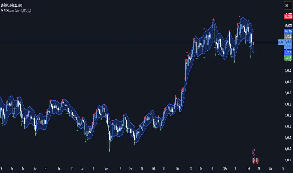
AE - ATR Exhaustion ChannelAE - ATR Exhaustion Channel
📈 Overview
Identify Exhaustion Zones & Trend Breakouts with ATR Precision!
The AE - ATR Exhaustion Channel is a powerful volatility-based trading tool that combines an averaged SMA with ATR bands to dynamically highlight potential trend exhaustion zones. It provides real-time breakout detection by marking when price moves beyond key volatility bands, helping traders spot overextensions and reversals with ease.
🔑 Key Features
✔️ ATR-SMA Hybrid Channel: Uses an averaged SMA as the core trend filter while incorporating adaptive ATR-based bands for precise volatility tracking.
✔️ Dynamic Exhaustion Markers: Marks red crosses when price exceeds the upper band and green crosses when price drops below the lower band.
✔️ Customizable ATR Sensitivity: Adjust the ATR multiplier and length settings to fine-tune band sensitivity based on market conditions.
✔️ Clear Channel Visualization: A gray SMA midpoint and a blue-filled ATR band zone make it easy to track market structure.
📚 How It Works
1️⃣ Averaged SMA Calculation: The script calculates an averaged SMA over a user-defined range (min/max period). This smooths out short-term fluctuations while preserving trend direction.
2️⃣ ATR Band Construction: The ATR value (adjusted by a multiplier) is added to/subtracted from the SMA to form dynamic upper and lower volatility bands.
3️⃣ Exhaustion Detection:
If high > upper ATR band, a red cross is plotted (potential overextension).
If low < lower ATR band, a green cross is plotted (potential reversal zone).
4️⃣ Filled ATR Channel: The area between the upper and lower bands is shaded blue, providing a visual trading range.
🎨 Customization & Settings
⚙️ ATR Length – Adjusts the ATR calculation period (default: 14).
⚙️ ATR Multiplier – Scales the ATR bands for tighter or wider volatility tracking (default: 0.8, adjustable in 0.1 steps).
⚙️ SMA Range (Min/Max Length) – Defines the period range for calculating the averaged SMA (default: 5-20).
⚙️ Rolling Lookback Length – Controls how far back the high/low comparison is calculated (default: 50 bars).
🚀 Practical Usage
📌 Spotting Exhaustion Zones – Look for red/green markers appearing outside the ATR bands, signaling potential trend exhaustion and possible reversal opportunities.
📌 Breakout Confirmation – Price consistently breaching the upper band with momentum could indicate continuation, while repeated touches without strong closes may hint at reversal zones.
📌 Trend Reversal Signals – Watch for green markers below the lower band in uptrends (buy signals) and red markers above the upper band in downtrends (sell signals).
🔔 Alerts & Notifications
📢 Set Alerts for Exhaustion Signals!
Traders can configure alerts to trigger when price breaches the ATR bands, allowing for instant notifications when volatility-based exhaustion is detected.
📊 Example Scenarios
✔ Trend Exhaustion in Overextended Moves – A series of red crosses near resistance may indicate a short opportunity.
✔ Trend Exhaustion in Overextended Moves – A series of red crosses near resistance may indicate an opportunity to open a short trade.
✔ Volatility Compression Breakouts – If price consolidates within the ATR bands and suddenly breaks out, it could signify a momentum shift.
✔ Reversal Catching in Trending Markets – Spot potential trend reversals by looking for green markers below the ATR bands in bullish markets.
🌟 Why Choose AE - ATR Exhaustion Channel?
Trade with Confidence. Spot Volatility. Catch Breakouts.
The AE - ATR Exhaustion Channel is an essential tool for traders looking to identify trend exhaustion, detect breakouts, and manage volatility effectively. Whether you're trading stocks, crypto, or forex, this ATR-SMA hybrid system provides clear visual cues to help you stay ahead of market moves.
✅ Customizable to Fit Any Market
✅ Combines Volatility & Trend Analysis
✅ Easy-to-Use with Instant Breakout Detection
Dynamic Deviation Levels [BigBeluga]Dynamic Deviation Levels is an innovative indicator designed to analyze price deviations relative to a smoothed midline. It provides traders with visual cues for overbought/oversold zones, price momentum, levels through labeled deviations and gradient candle coloring.
🔵Key Features:
Smoothed Midline:
A central line calculated as a smoothed median of the price source, serving as the baseline for price deviation analysis.
Dynamic Deviation Levels:
- Three deviation levels are plotted above and below the midline, with labels (1, 2, 3, -1, -2, -3) marking significant price movements.
- Helps traders identify overbought and oversold market conditions.
Heat-Colored Candles:
- Candle colors shift in intensity based on the deviation level, with four gradient shades for both upward and downward movements.
- Quickly highlights market extremes or stable zones.
Interactive Color Scale:
- A gradient scale at the bottom right of the chart visually represents deviation values.
- A triangle marker indicates the current price deviation in real time.
Optional Deviation Levels Display:
- Traders can enable all dynamic levels on the chart to visualize support and resistance areas dynamically.
🔵Usage and Benefits:
Identify Overbought/Oversold Zones: Use labeled deviation levels and heat-colored candles to spot stretched market conditions.
Track Trend Reversals and Momentum: Monitor price interactions with deviation levels for potential trend continuation or reversal signals.
Real-Time Deviation Insights: Leverage the color scale and triangle marker for live deviation tracking and actionable insights.
Map Dynamic Support and Resistance: Enable dynamic levels to highlight key areas where price reactions are likely to occur.
Dynamic Deviation Levels is an indispensable tool for traders aiming to combine price dynamics, momentum analysis, and visual clarity in their trading strategies.

E9 Bollinger RangeThe E9 Bollinger Range is a technical trading tool that leverages Bollinger Bands to track volatility and price deviations, along with additional trend filtering via EMAs.
The script visually enhances price action with a combination of trend-filtering EMAs, bar colouring for trend direction, signals to indicate potential buy and sell points based on price extension and engulfing patterns.
Here’s a breakdown of its key components:
Bollinger Bands: The strategy plots multiple Bollinger Band deviations to create different price levels. The furthest deviation bands act as warning signs for traders when price extends significantly, signaling potential overbought or oversold conditions.
Bar Colouring: Visual bar colouring is applied to clearly indicate trend direction: green bars for an uptrend and red bars for a downtrend.
EMA Filtering: Two EMAs (50 and 200) are used to help filter out false signals, giving traders a better sense of the underlying trend.
This combination of signals, visual elements, and trend filtering provides traders with a systematic approach to identifying price deviations and taking advantage of market corrections.
Brief History of Bollinger Bands
Bollinger Bands were developed by John Bollinger in the early 1980s as a tool to measure price volatility in financial markets. The bands consist of a moving average (typically 20 periods) with upper and lower bands placed two standard deviations away. These bands expand and contract based on market volatility, offering traders a visual representation of price extremes and potential reversal zones.
John Bollinger’s work revolutionized technical analysis by incorporating volatility into trend detection. His bands remain widely used across markets, including stocks, commodities, and cryptocurrencies. With the ability to highlight overbought and oversold conditions, Bollinger Bands have become a staple in many trading strategies.
Multi-Step FlexiSuperTrend - Indicator [presentTrading]This version of the indicator is built upon the foundation of a strategy version published earlier. However, this indicator version focuses on providing visual insights and alerts for traders, rather than executing trades. This one is mostly for @thorcmt.
█ Introduction and How it is Different
The **Multi-Step FlexiSuperTrend Indicator** is a versatile tool designed to provide traders with a highly customizable and flexible approach to trend analysis. Unlike traditional supertrend indicators, which focus on a single factor or threshold, the **FlexiSuperTrend** allows users to define multiple levels of take-profit targets and incorporate different trend normalization methods.
It comes with several advanced customization features, including multi-step take profits, deviation plotting, and trend normalization, making it suitable for both novice and expert traders.
BTCUSD 6hr Performance
█ Strategy, How It Works: Detailed Explanation
The **Multi-Step FlexiSuperTrend** works by calculating a supertrend based on multiple factors and incorporating oscillations from trend deviations. Here’s a breakdown of how it functions:
🔶 SuperTrend Calculation
At the heart of the indicator is the SuperTrend formula, which dynamically adjusts based on price movements.
🔶 Normalization of Deviations
To enhance accuracy, the **FlexiSuperTrend** calculates multiple deviations from the trend and normalizes them.
🔶 Multi-Step Take Profit Levels
The indicator allows setting up to three take profit levels, which are displayed via price level alerts. lows traders to exit part of their position at various profit intervals.
For more detail, please check the strategy version - Multi-Step-FlexiSuperTrend-Strategy:
and 'FlexiSuperTrend-Strategy'
█ Trade Direction
The **Multi-Step FlexiSuperTrend Indicator** supports both long and short trade directions.
This flexibility allows traders to adapt to trending, volatile, or sideways markets.
█ Usage
To use the **FlexiSuperTrend Indicator**, traders can set up their preferences for the following key features:
- **Trading Direction**: Choose whether to focus on long, short, or both signals.
- **Indicator Source**: The price source to calculate the trend (e.g., close, hl2).
- **Indicator Length**: The number of periods to calculate the ATR and trend (the larger the value, the smoother the trend).
- **Starting and Increment Factor**: These adjust how reactive the trend is to price movements. The starting factor dictates how far the initial trend band is from the price, and the increment factor adjusts subsequent trend deviations.
The indicator then displays buy and sell signals on the chart, along with alerts for each take-profit level.
Local picture
█ Default Settings
The default settings of the **Multi-Step FlexiSuperTrend** are carefully designed to provide an optimal balance between sensitivity and accuracy. Let’s examine these default parameters and their effect on performance:
🔶 Indicator Length (Default: 10)
The **Indicator Length** determines the lookback period for the ATR calculation. A smaller value makes the indicator more reactive to price changes, but may generate more false signals. A longer length smooths the trend and reduces noise but may delay signals.
Effect on performance: Shorter lengths perform better in volatile markets, while longer lengths excel in trending markets.
🔶 Starting Factor (Default: 0.618)
This factor adjusts the starting distance of the SuperTrend from the current price. The smaller the starting factor, the closer the trend is to the price, making it more sensitive. Conversely, a larger factor allows more distance, reducing sensitivity but filtering out false signals.
Effect on performance: A smaller factor provides quicker signals but can lead to frequent false positives. A larger factor generates fewer but more reliable signals.
🔶 Increment Factor (Default: 0.382)
The **Increment Factor** controls how the trend bands adjust as the price moves. It increases the distance of the bands from the price with each iteration.
Effect on performance: A higher increment factor can result in wider stop-loss or trend reversal bands, allowing for longer trends to develop without frequent exits. A lower factor keeps the bands closer to the price and is more suited for shorter-term trades.
🔶 Take Profit Levels (Default: 2%, 8%, 18%)
The default take-profit levels are set at 2%, 8%, and 18%. These values represent the thresholds at which the trader can partially exit their positions. These multi-step levels are highly customizable depending on the trader’s risk tolerance and strategy.
Effect on performance: Lower take-profit levels (e.g., 2%) capture small, quick profits in volatile markets, while higher levels (8%-18%) allow for a more gradual exit in strong trends.
🔶 Normalization Method (Default: None)
The default normalization method is **None**, meaning the deviations are not normalized. However, enabling normalization (e.g., **Max-Min**) can improve the clarity of the indicator’s signals in volatile or choppy markets by smoothing out the noise.
Effect on performance: Using a normalization method can reduce the effect of extreme deviations, making signals more stable and less prone to false positives.

itradesize /\ Previous Liquidity x ICTI’d like to introduce a clean and simple RTH gap and liquidity levels indicator with additional Asian and London ranges, along with standard deviation levels and many customizable options.
Previous D/W/M highs and lows are areas where liquidity tends to accumulate. This is because many traders place stop-loss orders around these levels, creating a concentration of buy stops above the previous day's high and sell stops below the previous day's low. High-frequency trading algorithms and institutional traders often target these areas to capture liquidity.
What the indicator could show in summary?
- Regular trading hours gap with deviations
- Asia with deviations (lines or boxes)
- London with deviations (lines or boxes)
- Weekdays on chart
- 3 AM candle marker
- Previous D/W/M levels
- Important opening times (08:00, 09:30, 10:00, 14:00, 00:00, 18:00)
- Daily separators
By marking out the previous day's highs and lows, traders can create a framework for their trading day. This helps in identifying potential setups and understanding where significant price action might occur. It also aids in filtering out noise and focusing on the most relevant price levels.
These levels can also act as potential reversal points. When the market reaches a previous high or low, it might reverse direction, especially if it has raided the liquidity resting there. This concept is part of a strategy where traders look for the market to raid these levels and then reverse, providing trading opportunities
The indicator shows previous liquidity levels on a daily, weekly, and monthly basis. It also displays opening times at 8:30, 9:30-10:00, 14:00-00:00, and 18:00. Opening times are crucial in trading because they help define specific periods when market activity is expected to be higher, which can lead to better trading opportunities. The script has been made mostly for indices.
You can create various entry and exit strategies based on the indicator. Please remember, that adequate knowledge of ICT is necessary for this to be beneficial.
You might wonder why only these times are shown. This is because these are the times when the futures market is active or should be active. It's important to note that opening times can vary between different asset classes.
18:00 A new daily candle open
00:00 Midnight open
02:00 New 4-hour candle open
08:30 High-impact news
09:30 NY Equities open
10:00 New 4-hour candle open
The concept of "Asian Killzone Standard Deviations" involves using the Asian trading session's price range to project potential price movements during subsequent trading sessions, such as the London or New York sessions. This is done by calculating standard deviations from the Asian range, which can help traders identify potential support and resistance levels.
You can create a complete model by exclusively focusing on the Asian time zone. Deviations within this zone may have varying impacts on future price movements, and the Interbank Price Delivery Agreement (IPDA) often reflects Asia's high, close, and low prices.
A similar approach can be taken with the London time zone. The standard deviation levels within each zone could potentially serve as support or indicate reversals, including liquidity hunts. It's important to backtest these ideas to gain reliable insights into when and where to apply them.
* Asian Range: This is the price range established during the Asian trading session. It serves as a reference point for calculating standard deviations.
* London Range: The same applies to the London range as well. Combine standard deviation projections with other technical analysis tools, such as order blocks or fair value gaps, to enhance accuracy.
* Standard Deviations: These are statistical measures that indicate the amount of variation or dispersion from the average. In trading, they are used to project potential price levels beyond the current range.
You can also use regular trading hours gap as a standalone model. The 4 STDV and 2.5 STDV levels are important for determining the high or low of the current price action.
The RTH gap is created when there is a difference between the closing price of a market at the end of one trading day and the opening price at the start of the next trading day. This gap can be upward (gap higher), downward (gap lower), or unchanged. It is significant because it often indicates market sentiment and can create inefficiencies that traders look to exploit.
Alternatively, you can combine these elements to create a complete strategy for different scenarios.