Breakout Targets [AlgoAlpha]🟠 OVERVIEW
This script identifies consolidation zones and provides automated breakout targets with risk management levels. It focuses on finding periods where price action compresses and then tracks the subsequent breakout from these ranges. When a price breakout is confirmed, the script automatically projects three take-profit (TP) levels and a stop-loss (SL) based on current market volatility. This helps traders move from identifying a range to executing a trade with predefined exit points without manual calculation.
🟠 CONCEPTS
The script uses a relationship between Weighted Moving Averages (WMA) and Exponential Moving Averages (EMA) of price ranges to detect consolidation. When these moving averages cross, it triggers the detection of recent pivot highs and lows to draw a visual "box" or channel. This channel represents the current trading range. Once price closes outside this box, the script uses the Average True Range (ATR) to determine the volatility-adjusted distance for the stop loss. The take-profit levels are then calculated as multiples of this risk distance, ensuring a consistent reward-to-risk approach.
🟠 FEATURES
Dynamic box drawing that highlights potential supply and demand zones within the range.
Real-time breakout signals with bullish (green) and bearish (red) markers.
Automated trade projection including Entry, SL, and three TP levels.
Integrated alert system for breakouts and hits on any profit or loss target.
🟠 USAGE
Setup : Add the script to your chart and adjust the "Range Detection Period." A higher period will find larger, more significant ranges, while a lower period will find smaller, short-term consolidation zones.
Read the chart : Look for the grey boxes on your chart; these represent areas where the market is "coiling." A green arrow label indicates a bullish breakout from the top of the box, while a red arrow indicates a bearish breakout from the bottom. Once a breakout occurs, follow the projected horizontal levels for your trade management.
Settings that matter : The Stop Loss ATR Multiplier is the most critical setting for risk; increasing it will give the trade more room to breathe but will also push your TP levels further away. The Prevent Overlap toggle is useful for keeping the chart clean by ensuring the script doesn't draw new boxes until the current range has been resolved.
Trendfollowing

Adaptive RSIAdaptive RSI
Adaptive RSI is an enhanced version of the classic Relative Strength Index designed to automatically adjust its behavior to changing market conditions. The indicator can operate both as a mean-reversion oscillator and as a trend-following momentum tool, allowing traders to detect high/low value zones while also capturing directional moves.
Unlike the traditional RSI, which uses a fixed smoothing method, Adaptive RSI dynamically changes its calculation speed depending on market activity. This helps reduce false signals in slow or choppy markets while allowing faster responses during strong moves.
🔍 Concept & Idea
The goal behind Adaptive RSI is to make RSI responsive when opportunities appear and more conservative during uncertain or low-activity environments.
By automatically adjusting its internal smoothing and reaction speed, the indicator attempts to balance:
• Early entries during strong market moves
• Reduced noise during consolidation
• Mean-reversion opportunities in ranging markets
• Momentum confirmation in trending markets
This adaptive behavior makes the oscillator more versatile across multiple market conditions.
⚙️ How It Works
The indicator evaluates market activity using three drivers:
• True Range (volatility)
• Volume activity
• Rate of price change
Users can define which of these factors has priority. The script then checks up to three conditions; the more conditions that are satisfied, the faster and more responsive the RSI calculation becomes.
This creates multiple internal speed tiers ranging from smooth and conservative to highly responsive.
After the adaptive RSI is calculated, an additional adaptive smoothing layer is applied using the same logic, improving signal clarity while preserving responsiveness.
An optional feature allows the RSI to use a special Rate-of-Change weighted price source. This feature is more advanced and mainly intended for users who understand how weighted price construction affects oscillators.
A divergence measure between the base RSI and the smoothed Adaptive RSI is also plotted to help visualize shifts in momentum strength.
⚙️ Key Features
• Adaptive RSI calculation speed
• Works for both trend-following and mean-reversion approaches
• Adjustable long and short signal thresholds
• Overbought and oversold zone highlighting
• Divergence histogram between RSI and adaptive smoothing
• Trend-based coloring and visual signal markers
• Optional ROC-weighted source for advanced users
🧩 Inputs Overview
• RSI calculation length and smoothing length
• Price source selection or optional special weighted source
• Speed tier selection (slow, medium, fast behavior)
• Activity priority order (volatility, volume, momentum)
• Long/short and overbought/oversold thresholds
📌 Usage Notes
• Can be used both for trend continuation and mean-reversion strategies.
• Adaptive logic helps reduce noise during sideways markets.
• Strong moves may cause faster RSI transitions due to adaptive speed selection.
• Signals may update intrabar on lower timeframes.
• Works best when combined with risk management and confirmation tools.
• No indicator is perfect; always test before live use.
This script is intended for analytical purposes only and does not provide financial advice.

Smart SafeZone Stops [MarkitTick]💡 This script represents a sophisticated evolution of volatility-based trailing stop methodologies. It is designed to assist traders in managing trend-following positions by dynamically adjusting stop-loss levels based on market noise, directional momentum, and volume flows. Unlike static trailing stops that move by a fixed percentage or simple ATR multiples, this tool calculates the "safe zone" by analyzing how far price has penetrated against the trend over a specific lookback period, offering a granular approach to risk management that adapts to changing market conditions.
✨ Originality and Utility
The primary utility of this indicator lies in its ability to filter out market noise while remaining tight enough to protect profits during strong trends. While the classic SafeZone concept (popularized by Dr. Alexander Elder) is effective, this script introduces several modern enhancements that increase its robustness:
● Dynamic ADX Integration Standard SafeZone stops use a fixed multiplier. This script integrates the Average Directional Index (ADX) to gauge trend strength. When the trend is strong, the stop tightens (Aggressive Multiplier) to lock in profits rapidly. When the trend is weak or choppy, the stop widens (Conservative Multiplier) to prevent premature shakeouts. ● Volume-Weighted Noise Price movement on low volume is often considered "noise," while high-volume movement signifies conviction. This script optionally weights the noise calculation by Relative Volume. A downward spike on low volume will affect the stop level less than a downward spike on high volume.
● 3-Day Smoothing Mechanism To prevent the stop line from becoming too jagged or reacting to single-bar anomalies, the script applies a 3-day smoothing algorithm. It utilizes the "worst-case" scenario of the last three calculated stop levels, ensuring the stop only moves when the trend structure genuinely shifts.
🔬 Methodology and Concepts
The underlying logic operates on a "Ratchet" mechanism, meaning the stop line can only move in the direction of the trade (up for longs, down for shorts) and never retraces until a trend reversal occurs.
● Directional Noise Calculation The script separates market noise into two components: Downside Penetration (for Longs): The distance the price dips below the previous bar's low. Upside Penetration (for Shorts): The distance the price spikes above the previous bar's high. The average of these penetrations is calculated over the Noise Lookback Period .
● The SafeZone Formula The raw stop level is derived as follows: Long Stop = Previous Low - (Average Downside Noise × Multiplier) Short Stop = Previous High + (Average Upside Noise × Multiplier)
● Adaptive Multiplier Logic If Dynamic ADX is enabled: If ADX > Strong Threshold: Use Aggressive Multiplier (e.g., 1.5x). If ADX < Weak Threshold: Use Conservative Multiplier (e.g., 3.5x). Otherwise: Use the Base Safety Coefficient.
● Exhaustion Detection The script calculates the distance between the current Close price and the Active Stop. If this distance exceeds a specific multiple of the ATR (Average True Range), it flags a "Mean Reversion" or "Exhaustion" warning, suggesting price has extended too far from equilibrium.
🎨 Visual Guide
The indicator plots distinct visual elements to guide decision-making without cluttering the chart excessively.
● Trailing Stop Lines Green Line (Solid): Represents the SafeZone Long Stop. This line appears below price during an uptrend. As long as price closes above this line, the bullish bias is intact. Red Line (Solid): Represents the SafeZone Short Stop. This line appears above price during a downtrend. A close above this line signals a potential short exit or reversal.
● Trend Signals Green Triangle (Below Bar): Marks the "Bull Start." This occurs when the price crosses above the Trend Filter EMA and the trend logic flips to bullish. Red Triangle (Above Bar): Marks the "Bear Start." Indicates the start of a downtrend sequence.
● Exhaustion Warnings Yellow Labels (⚠️): These appear when price has extended significantly away from the stop line (based on the ATR Exhaustion Multiplier). This is not an immediate sell signal but a warning that the trend may be overextended and a pullback is probable.
● MTF Consensus Cloud Background Color: If enabled, the chart background changes color to reflect the Higher Timeframe (HTF) trend. Green Background: Current trend matches HTF Uptrend. Red Background: Current trend matches HTF Downtrend. Gray Background: Trends are mismatched (Consolidation/Conflict).
● Quantitative Dashboard A table located in the top-right corner displays real-time statistics: Trend: Current state (BULLISH/BEARISH). Age: Number of bars since the trend began. Stop Price: Exact price level of the trailing stop. Risk %: The percentage distance from the current Close to the Stop. If this exceeds 3%, the text turns red to highlight elevated risk. Active Mult: The current multiplier being used (Dynamic or Fixed). ADX State: Shows if the trend is Strong, Weak, or Normal.
📖 How to Use
1. Entry Timing Wait for a Trend Switch signal (Triangle). For a long entry (Green Triangle), ensure the price is above the Trend Baseline (EMA). Ideally, look for confluence with the MTF Cloud (Green Background).
2. Position Management Once in a trade, use the Trailing Stop Line as your hard exit or invalidation point. Do not manually move the stop away from price; the script automatically "ratchets" the stop tighter as the trend progresses.
3. Taking Profits Use the "Exhaustion Warnings" (⚠️) as opportunities to scale out of positions. When price moves parabolically away from the stop line, the probability of a snap-back increases.
4. Managing Chop If the dashboard shows "ADX State: WEAK," expect the stop line to remain wider. This allows the asset "room to breathe" without stopping you out on random volatility.
⚙️ Inputs and Settings
The script is highly customizable to fit different asset classes (Crypto, Forex, Stocks).
● Trend Definitions Trend Filter (EMA Length): Determines the baseline trend bias (Default: 22). Price must be above this EMA to initiate a long calculation.
● Noise Calculation Noise Lookback Period: The number of bars used to calculate average penetration (Default: 10). Base Safety Coefficient: The standard multiplier applied to the noise average (Default: 2.5). Higher values = wider stops. Use Volume Weighting: Enables the volume-adjustment logic. Use 3-Day Smoothing: Recommended keeping this TRUE to avoid stop-hunts.
● Dynamic Multiplier (ADX) Enable Dynamic ADX: Toggles the adaptive multiplier. Strong/Weak Thresholds: The ADX levels that trigger aggressive or conservative multipliers.
● Multi-Timeframe Consensus Higher Timeframe: Select the TF for the cloud background (e.g., Daily or Weekly).
● Exhaustion Warning ATR Multiplier: Defines how far price must be from the stop to trigger a warning (Default: 3.0).
🔍 Deconstruction of the Underlying Scientific and Academic Framework
The "Smart SafeZone" indicator is grounded in the statistical analysis of market noise versus signal.
● Theory of Noise Penetration Conventional stops often use Standard Deviation (Bollinger Bands) or Average True Range (Keltner Channels/Chandelier Stops). While effective, these measures assume volatility is symmetrical. This script adopts the view that directional volatility matters more. In an uptrend, upside volatility is "good" signal, while downside volatility is "noise." By explicitly calculating the average downside penetration (Low - Low), the script isolates the specific counter-trend force acting on the asset. ● Volume-Weighted Price Analysis (VWPA) The inclusion of volume weighting draws upon Dow Theory principles, which state that volume must confirm the trend. Math: Penetration × (Volume / AverageVolume) This formula asserts that a price drop on low volume is statistically less significant than a drop on high volume. By dampening the impact of low-volume moves, the stop becomes more resistant to liquidity vacuums and algorithmic stop-hunts.
● Trend Efficiency (ADX) The integration of J. Welles Wilder’s ADX (Average Directional Index) adds a dimension of Trend Efficiency. High ADX values indicate a highly efficient trend with little retracement. Mathematically, this justifies a lower standard deviation (or noise multiplier) for the stop, as the probability of a deep retracement without a trend change is lower in high-momentum environments.
⚠️ Disclaimer
All provided scripts and indicators are strictly for educational exploration and must not be interpreted as financial advice or a recommendation to execute trades. I expressly disclaim all liability for any financial losses or damages that may result, directly or indirectly, from the reliance on or application of these tools. Market participation carries inherent risk where past performance never guarantees future returns, leaving all investment decisions and due diligence solely at your own discretion.

Cyberpunk Vortex IndicatorCyberpunk Vortex Indicator is a visually enhanced Vortex-based momentum indicator designed to clearly capture trend strength and directional dominance.
This indicator calculates VI+ (bullish pressure) and VI− (bearish pressure) using the classic Vortex methodology, then renders them with a layered neon cyberpunk-style glow for maximum readability and impact.
🔹 Key Features
・Vortex Indicator (VI+ / VI−) with SMA smoothing
・Multi-layer laser-style glow (outer / inner / core lines)
・Clear visual distinction between bullish and bearish momentum
・Subtle background and fill effects for intuitive trend recognition
・Clean, modern design without clutter
🔹 How to Use
・VI+ above VI− → Bullish momentum dominates
・VI− above VI+ → Bearish momentum dominates
・The 1.0 baseline helps identify strengthening or weakening trends
・Best used as a trend confirmation tool, not a standalone signal
🔹 Recommended Timeframes
Works well across multiple timeframes.
Commonly effective on 15m, 1H, 4H, and higher.
This indicator focuses on clarity, aesthetics, and momentum visualization, making it ideal for traders who value both performance and design.
Cyberpunk Vortex Indicator は、トレンドの強さと方向性を直感的に把握するために設計された、視認性とデザイン性を重視したボルテックス系モメンタム指標です。
クラシックな Vortex Indicator(VI+ / VI−)をベースに、サイバーパンク調のネオン発光レイヤーで描画することで、買い圧力・売り圧力の優位性を一目で判断できます。
🔹 特徴
・Vortex Indicator(VI+ / VI−)をSMAでスムージング
・外側・内側・芯の3層レーザー風グロー表現
・上昇 / 下降モメンタムの視認性を大幅に向上
・控えめな背景・塗りつぶしで相場の空気感を演出
・ノイズの少ない、洗練されたデザイン
🔹 使い方
・VI+ が VI− を上回る → 上昇トレンド優勢
・VI− が VI+ を上回る → 下降トレンド優勢
・1.0 の基準線でトレンドの勢いを確認
・単体判断ではなく、トレンド確認用としての使用を推奨
🔹 推奨時間足
マルチタイムフレーム対応。
特に 15分足 / 1時間足 / 4時間足以上で安定。
本インジケーターは
「見やすさ」「美しさ」「モメンタムの可視化」を重視しており、
デザインと実用性の両立を求めるトレーダー向けです。

Sigmoid Risk AllocatorThe Sigmoid Risk Allocator is a dynamic position sizing indicator that tells you how much of your capital to allocate based on current market conditions. Unlike simple "risk-on/risk-off" signals, this indicator gives you smooth, gradual transitions based on a sigmoid function.
Why a Sigmoid Curve?
Most position sizing approaches use fixed thresholds: "If drawdown > 20%, buy. Otherwise, don't." This creates all-or-nothing decisions.
Using the sigmoid (S-curve) makes this decision different. It creates a smooth transition where:
Small drawdowns → Stay near your baseline allocation
Moderate drawdowns → Gradually increase exposure
Large drawdowns → Approach maximum allocation
The sigmoid curve naturally "saturates" at the extremes, preventing you from going all-in too early or panicking out too fast. This is very useful to meek traders psychology and risk management in check.
What's a Sigmoid Function?
The sigmoid function is a mathematical S-curve defined as:
σ(x) = 1 / (1 + e^(-x))
This formula takes any input value and smoothly maps it to a number between 0 and 1. The curve has three key properties that make it ideal for position sizing in investing:
Smooth transitions: No sudden jumps. Allocation changes gradually.
Saturation at extremes: The curve flattens near 0 and 1, preventing overreaction and overexposure.
Sensitive in the middle: Most of the action happens around the midpoint.
To convert this into an allocation percentage, the indicator uses:
Allocation = α_min + (α_max - α_min) × σ(k × (Risk - Midpoint))
Where:
- `α_min` = Your minimum allocation (default 50%)
- `α_max` = Your maximum allocation (default 100%)
- `Risk` = Current risk metric (drawdown %, volatility, or Kelly %)
- `Midpoint` = The risk level where allocation sits halfway between min and max (default 15%)
- `k` = Steepness—how quickly allocation changes around the midpoint
Example : With defaults, if drawdown hits 15% (the midpoint), your allocation will be 75% (halfway between 50% and 100%). As the drawdown increases beyond 15%, the allocation curves toward 100%. As it decreases toward 0%, allocation curves toward 50%.
Cool, isn't it?
Asymmetric Response: Fast In, Slow Out
The indicator uses different steepness values for scaling in vs. scaling out. This is great to increase trend following. This is something I'm proud of too in this indicator.
k_increase = 30 (steep curve): When drawdowns appear, allocation ramps up quickly to catch the opportunity
k_decrease = 5 (slower curve): When conditions normalize, allocation decreases slowly to avoid selling the rebound
This asymmetry reflects how markets behave—drawdowns often overshoot fundamentals (rewarding quick entries), while recoveries tend to be more orderly (rewarding patience on exits).
Three Risk Metrics
You can choose what drives your allocation:
Drawdown (Default)
Volatility - Scales your position inversely to current market volatility.
Kelly Criterion - Automatically calculates optimal position size. The indicator applies a conservative "half Kelly" by default.
Use Cases
Position sizing for swing trading or trend following
Risk management overlay for any existing strategy
Drawdown-based DCA (dollar cost averaging) decisions
Volatility-adjusted exposure management
Feel free to provide feedback and share your thoughts!
- Henrique Centieiro

House Rules SuperTrend Strategy (ATR-Based, Non-Repainting)📝 DESCRIPTION
Overview
The House Rules SuperTrend Strategy is a clean, rule-based trading strategy built using Pine Script® v6.
It is designed for transparent backtesting, non-repainting signals, and simple trend-following execution across all markets and timeframes.
This strategy uses TradingView’s built-in SuperTrend indicator, which is derived from Average True Range (ATR), to identify trend direction changes and generate long and short trades.
How the Strategy Works
Long Entry
A long position is opened when the SuperTrend flips from bearish to bullish
This confirms a potential upward trend shift
Short Entry
A short position is opened when the SuperTrend flips from bullish to bearish
This confirms a potential downward trend shift
Exits
Positions are closed when either:
The opposite SuperTrend signal appears, or
The ATR-based Stop Loss or Take Profit is reached (if enabled)
All signals are calculated on confirmed candle closes only, ensuring accurate and fair backtesting.
Risk Management
Optional ATR-based Stop Loss
Optional ATR-based Take Profit
Position sizing based on percentage of equity
Commission included for realistic performance results
All parameters are user-adjustable from the settings panel.
Backtesting & Transparency
This is a strategy, not an indicator
No repainting
No future data usage
No hidden filters
No lookahead bias
Fully compatible with TradingView’s Strategy Tester
Users are encouraged to test different symbols, timeframes, and parameter values to suit their trading style.
Recommended Use
This strategy can be used on:
Cryptocurrencies
Forex
Stocks
Indices
Futures
It performs best in trending market conditions and may underperform during low-volatility or ranging markets.
Disclaimer
This script is provided for educational and research purposes only.
It is not financial advice. Always test and validate strategies before using them in live trading.

MAD Supertrend [Alpha Extract]A sophisticated SuperTrend implementation that replaces traditional ATR calculations with Mean Absolute Deviation methodology for adaptive volatility measurement and band construction. Utilizing SMA baseline with MAD-based deviation bands and optional adaptive factor adjustments, this indicator delivers institutional-grade trend detection with strength-based filtering and dynamic visual feedback. The system's MAD approach provides superior noise reduction compared to ATR while maintaining responsiveness to genuine volatility changes, combined with momentum-based strength calculations for high-conviction signal generation.
🔶 Advanced MAD-Based Band Construction
Implements Mean Absolute Deviation calculation as volatility proxy, measuring absolute price deviations from mean and smoothing for stable band generation without ATR dependency. The system calculates SMA baseline, computes MAD from configurable lookback period, applies factor multipliers to create upper and lower bands, then implements classic SuperTrend ratcheting logic where bands only adjust when price violates previous levels or calculations warrant updates.
// Core MAD SuperTrend Framework
SMA_Value = ta.sma(src, SMA_Length)
Mean = ta.sma(src, MAD_Length)
Abs_Deviation = abs(src - Mean)
MAD_Value = ta.sma(Abs_Deviation, MAD_Length)
// Band Construction with Ratcheting
Upper_Band = SMA_Value + MAD_Factor * MAD_Value
Lower_Band = SMA_Value - MAD_Factor * MAD_Value
// Ratcheting logic prevents premature band adjustments
🔶 Adaptive Factor Adjustment Engine
Features optional adaptive multiplier system that modulates MAD factor based on normalized MAD magnitude relative to recent extremes, creating bands that automatically expand during high-volatility regimes and contract during consolidation. The system applies min-max normalization to MAD values over configurable lookback, multiplies by adaptation parameter, and adds to base factor for dynamic volatility sensitivity without manual recalibration.
🔶 Momentum-Based Strength Filter
Implements sophisticated strength calculation measuring price momentum relative to baseline divided by volatility-adjusted MAD bands, producing normalized 0-1 strength scores with exponential smoothing. The system calculates distance from SMA baseline, normalizes by MAD-derived band width, and applies configurable minimum threshold requiring sufficient momentum before trend signals activate, filtering weak or choppy market conditions.
🔶 SuperTrend Direction Logic
Utilizes classic SuperTrend methodology adapted for MAD bands where trend direction flips on opposite band violations with state persistence until confirmation. The system tracks whether price closes above upper band (bearish flip to bullish) or below lower band (bullish flip to bearish), maintains directional state until opposing violation occurs, and generates binary +1/-1 trend signals suitable for systematic position management.
🔶 Intelligent Candle Sticking System
Provides advanced line positioning option that anchors SuperTrend line to candle wicks or bodies rather than pure calculation values for enhanced visual clarity. The system supports two modes: Wick (positions at high/low extremes based on trend direction) and Body (constrains line between calculation and candle extremes), creating cleaner chart presentation while maintaining mathematical integrity of underlying signals.
🔶 Dynamic Gradient Visualization Framework
Implements color intensity modulation based on smoothed strength calculations, transitioning from muted to vivid hues as momentum conviction increases. The system applies gradient interpolation using strength ratio, creating visual feedback where strong trending moves display intense colors while weak or consolidating conditions show faded tones across trend line, channel bands, and candle coloring for immediate regime assessment.
🔶 MAD Channel Architecture
Features volatility-adjusted channel bands centered on baseline or candle-stuck line with configurable multiplier for support/resistance visualization. The system calculates upper and lower bounds using MAD values scaled by adaptive factors and channel multipliers, applies dynamic transparency based on trend strength, and creates filled regions that intensify during strong trends and fade during weak conditions.
🔶 Multi-Layer Glow Effect System
Provides sophisticated line rendering with triple-layer plot system creating glow effect through progressively wider and more transparent outer layers. The system plots core trend line at specified width with full color intensity, adds inner glow layer at +2 width with moderate transparency, and outer glow at +4 width with higher transparency, creating visual depth and emphasis without cluttering chart space.
🔶 Strength-Based State Management
Implements intelligent trend state logic requiring both directional signal and minimum strength threshold breach before confirming trend transitions. The system calculates raw SuperTrend direction, evaluates smoothed strength against configurable minimum, generates filtered trend state that can be bullish (+1), bearish (-1), or neutral (0), and maintains state persistence using hold logic that prevents oscillation during ambiguous conditions.
🔶 Comprehensive Alert Integration
Generates trend flip alerts when filtered state transitions from bearish to bullish or bullish to bearish with full confirmation requirements satisfied. The system detects state changes through comparison with previous bar, triggers single alert per transition rather than continuous notifications, and provides customizable message templates for automated trading system integration or manual notification preferences.
🔶 Performance Optimization Architecture
Utilizes efficient calculation methods with null value handling, nz() functions preventing errors during initialization bars, and optimized gradient calculations. The system includes intelligent state persistence minimizing recalculation overhead, streamlined MAD computation avoiding redundant mean calculations, and smooth visual updates maintaining consistent performance across extended historical periods.
This indicator delivers sophisticated SuperTrend analysis through Mean Absolute Deviation methodology providing superior statistical properties compared to traditional ATR-based approaches. MAD calculations offer more robust volatility measurement resistant to extreme outliers while maintaining sensitivity to genuine market regime changes. The system's adaptive factor adjustment, momentum-based strength filtering, and dynamic visual feedback make it essential for traders seeking reliable trend-following signals with reduced false breakouts during choppy conditions. The combination of MAD bands, candle-sticking options, gradient strength visualization, and comprehensive filtering creates institutional-grade trend detection suitable for systematic approaches across cryptocurrency, forex, and equity markets with clear entry/exit signals and comprehensive alert capabilities.

Smart Money Volume Index [AlgoAlpha]🟠 OVERVIEW
This script measures buying and selling interest by comparing how price behaves on rising volume versus falling volume. It separates what is often called “smart money” activity from more passive volume and turns that relationship into a normalized index. The result is an oscillator that shows whether buyers or sellers are in control, how strong that control is, and when interest reaches extreme levels that tend to matter for reversals or continuations.
🟠 CONCEPTS
The calculation starts by splitting volume flow into two streams. Positive Volume Index (PVI) reacts when volume expands, while Negative Volume Index (NVI) reacts when volume contracts. Each stream is detrended with a long EMA and passed through an RSI calculation to express relative pressure. These two RSIs are then compared as ratios to estimate buy-side and sell-side interest. The values are summed over a rolling window and normalized against historical peaks so the output stays bounded and comparable across markets. In simple terms: relative behavior on high-volume vs low-volume bars defines interest , and normalization makes that interest readable over time.
🟠 FEATURES
Two display modes: Compare (separate buy and sell interest) and Net (single combined oscillator)
High-interest threshold zones with visual highlights
Alert conditions for threshold crosses and zero-line shifts
🟠 USAGE
Setup : Add the script to your chart. Choose Net mode for a clean momentum-style read, or Compare mode to see buy and sell interest separately. Start with the default periods, then adjust the Index Period to control how much history is included.
Read the chart : Values above zero mean buy-side interest dominates; below zero means sell-side interest dominates. In Compare mode, the green line tracks buying interest and the red line tracks selling interest. When either side pushes beyond the high-interest threshold, participation is elevated and moves tend to be more meaningful.
Settings that matter : Increasing the Index Period smooths the index and focuses on longer participation trends. Changing the Volume Flow Period alters how sensitive the RSI-based pressure is. The High Interest Threshold controls how selective extreme signals are and directly affects alerts and zone highlights.

SMC Alpha Engine [PhenLabs]📊 SMC Alpha Engine
Version: PineScript™ v6
📌 Description
The SMC Alpha Engine is a comprehensive Smart Money Concepts indicator that automates institutional trading pattern recognition. Built for traders who understand that confluence is king, this indicator stacks multiple SMC elements together and scores them in real-time, allowing you to focus exclusively on high-probability setups.
Rather than manually tracking HTF bias, market structure, liquidity levels, order blocks, and fair value gaps separately, the SMC Alpha Engine consolidates everything into a unified scoring system. When enough factors align, you get a signal. When they don’t, you wait. This systematic approach removes emotion and subjectivity from SMC trading.
The indicator is designed around one core principle: only trade when the probabilities are stacked in your favor. By requiring multiple confluence factors before generating signals, it filters out the noise and keeps you focused on setups that institutional traders actually care about.
🚀 Points of Innovation
Automated confluence scoring system that evaluates 6 distinct SMC factors in real-time
HTF-to-LTF bias alignment ensuring trades flow with institutional direction
Intelligent liquidity sweep detection using wick-ratio analysis for confirmation
ATR-based FVG quality filtering that eliminates noise and shows only significant imbalances
Anti-spam signal logic preventing overtrading during volatile market conditions
Session-aware killzone integration timing entries with institutional activity windows
🔧 Core Components
HTF Bias Engine: Analyzes higher timeframe swing structure to establish directional bias using pivot high/low comparisons
Market Structure Module: Detects BOS (Break of Structure) and CHoCH (Change of Character) with real-time confirmation
Premium/Discount Calculator: Dynamically maps price zones relative to recent swing range equilibrium
Liquidity Tracker: Monitors swing points as liquidity targets and identifies sweep events with rejection confirmation
POI Detector: Identifies valid Order Blocks with displacement requirements and Fair Value Gaps with ATR filtering
Confluence Scorer: Aggregates all factors into bull/bear scores displayed on real-time dashboard
🔥 Key Features
Multi-timeframe analysis combining HTF directional bias with LTF precision entries
Customizable confluence threshold from 1 (low filter) to 5 (sniper mode)
Three killzone sessions: London (02:00-05:00), NY AM (08:30-11:00), NY PM (13:30-16:00)
Flexible mitigation options for OBs and FVGs: Wick, Close, 50%, or None
Visual structure labeling for BOS and CHoCH events on chart
Real-time info dashboard showing all current market conditions and scores
Built-in alert conditions for BOS, liquidity sweeps, and high-confluence signals
🎨 Visualization
Premium Zone: Red-tinted box above equilibrium indicating sell-side interest areas
Discount Zone: Green-tinted box below equilibrium indicating buy-side interest areas
Equilibrium Line: Dotted gray line marking the 50% level of current range
Order Blocks: Color-coded boxes (green for bullish, red for bearish) showing institutional candles
Fair Value Gaps: Teal boxes for bullish FVGs, maroon boxes for bearish FVGs
Killzone Backgrounds: Blue (London), Orange (NY AM), Purple (NY PM) session highlighting
Info Table: Top-right dashboard displaying HTF bias, LTF trend, zone, killzone status, and scores
📖 Usage Guidelines
HTF Settings
HTF Timeframe - Default: 60 - Controls higher timeframe for directional bias
HTF Swing Length - Default: 10, Range: 3+ - Determines pivot sensitivity for HTF trend
Market Structure Settings
LTF Swing Length - Default: 3, Range: 1-10 - Controls swing detection sensitivity
Show BOS/CHoCH - Default: Off - Toggles structure labels on chart
Show Strong/Weak Points - Default: Off - Displays swing point classifications
POI Settings
Show Valid Order Blocks - Default: Off - Displays OBs that caused displacement
Show Unmitigated FVGs - Default: On - Shows active fair value gaps
Filter FVG by ATR - Default: On - Only shows FVGs larger than 0.5x ATR
OB Mitigation Type - Options: Wick, Close, None - Determines when OBs are invalidated
FVG Mitigation Type - Options: Wick, Close, 50%, None - Determines when FVGs are filled
Confluence Settings
Minimum Score for Signal - Default: 4, Range: 1-5 - Required confluence level for entries
Show Entry Signals - Default: On - Toggles LONG/SHORT labels on chart
✅ Best Use Cases
Trend continuation trades during active killzone sessions with HTF alignment
Discount zone entries on bullish HTF bias with recent liquidity sweep below
Premium zone shorts on bearish HTF bias after liquidity grab above recent highs
Reversal identification following CHoCH with POI confluence in optimal zone
Filtering existing strategy signals by requiring minimum confluence score
⚠️ Limitations
HTF bias detection requires sufficient price history for accurate pivot identification
Liquidity sweep detection depends on wick-ratio settings and may miss some events
Order blocks require displacement confirmation which may exclude some valid zones
Confluence scoring is probabilistic and does not guarantee profitable outcomes
Killzone times are based on EST/EDT and require timezone adjustment for other regions
Signal spam prevention may delay valid signals by up to 10 bars after previous signal
💡 What Makes This Unique
Unified SMC Framework: Combines all major SMC concepts into one cohesive indicator rather than requiring multiple tools
Objective Scoring System: Removes subjectivity by quantifying confluence into measurable scores
Institutional Timing Integration: Built-in killzone awareness ensures signals align with high-volume sessions
Quality Filtering: ATR-based FVG filtering and displacement-required OBs eliminate low-quality setups
Anti-Overtrading Logic: Smart signal spacing prevents emotional trading during choppy conditions
🔬 How It Works
Step 1: HTF Bias Determination
Analyzes higher timeframe pivot highs and lows
Compares consecutive pivots to identify HH/HL (bullish) or LH/LL (bearish) sequences
Establishes directional filter that all signals must respect
Step 2: LTF Structure Mapping
Detects swing points on execution timeframe
Identifies BOS when price closes beyond confirmed swing level
Recognizes CHoCH when structure break occurs against current trend
Step 3: Confluence Calculation
Awards +1 for HTF bias alignment
Awards +1 for active killzone timing
Awards +1 for optimal zone positioning (discount for longs, premium for shorts)
Awards +1 for price at unmitigated POI
Awards +1 for recent liquidity sweep in trade direction
Awards +1 for recent supportive structure break
Step 4: Signal Generation
Compares total score against user-defined minimum threshold
Requires candle confirmation (bullish close for longs, bearish close for shorts)
Applies 10-bar spacing filter to prevent signal clustering
💡 Note:
This indicator is designed for traders already familiar with Smart Money Concepts. While it automates detection and scoring, understanding why each factor matters will significantly improve your ability to filter signals and manage trades effectively. Use the minimum confluence setting to match your risk tolerance, higher values mean fewer but higher-quality signals.

Volume-Adjusted CCI Trend [Alpha Extract]A sophisticated trend identification system that combines dual EMA direction analysis with volume-weighted normalization and CCI momentum filtering for comprehensive trend validation. Utilizing Volume RSI integration and standard deviation-based bands that expand and contract with volume characteristics, this indicator delivers institutional-grade trend detection with multi-layered confirmation requirements. The system's volume adjustment mechanism modulates signal sensitivity based on participation strength while CCI thresholds prevent false signals during weak momentum conditions, creating a robust trend-following framework with reduced whipsaw susceptibility.
🔶 Advanced Dual EMA Direction Engine
Implements fast and slow exponential moving average comparison to establish primary trend direction bias with configurable period parameters for timeframe optimization. The system calculates trend direction as binary +1 (bullish when fast EMA exceeds slow EMA) or -1 (bearish when slow exceeds fast), providing foundational directional input that requires additional confirmation before generating actionable trend states.
🔶 Volume-Adjusted Normalization Framework
Features sophisticated normalization calculation that measures price deviation from basis EMA, scales by standard deviation, then applies volume-weighted adjustment factor for participation-sensitive signal generation. The system calculates Volume RSI to quantify relative volume strength, converts to ratio format, and multiplies normalized deviation by volume factor scaled by impact parameter, creating signals that strengthen during high-volume confirmations and weaken during low-volume moves.
// Volume-Adjusted Normalization
Vol_Ratio = Volume_RSI / 50
Vol_Factor = 1 + (Vol_Ratio - 1) * Vol_Impact
Dev = src - Basis_EMA
Raw_Normalized = Dev / (StdDev * Multiplier)
Vol_Adjusted_Norm = Raw_Normalized * Vol_Factor
🔶 CCI Momentum Filter Integration
Implements Commodity Channel Index threshold system with configurable upper and lower bounds to validate trend strength and filter sideways market conditions. The system calculates standard CCI with adjustable length, compares against asymmetric thresholds (default +100 bullish, -50 bearish), and requires CCI confirmation in addition to EMA direction and normalized deviation before transitioning trend states, ensuring only high-conviction signals generate entries.
🔶 Multi-Layer Trend State Logic
Provides intelligent trend state machine requiring simultaneous confirmation from EMA direction, volume-adjusted normalization threshold breach, and optional CCI momentum validation. The system maintains persistent trend state that only transitions when all three conditions align, preventing premature reversals during temporary retracements or low-volume fluctuations while capturing genuine trend changes with institutional-grade confirmation requirements.
🔶 Dynamic Volume Band Architecture
Creates volatility-adjusted bands around basis EMA using standard deviation multiplied by volume factor, producing channels that widen during high-volume periods and contract during low-volume consolidations. The system applies identical volume adjustment to band calculations as normalization metric, ensuring visual envelope consistency with underlying signal logic and providing intuitive reference boundaries for trend-following price action.
🔶 Gradient Strength Visualization System
Implements color intensity modulation based on normalized signal strength relative to threshold requirements, creating visual feedback that communicates trend conviction. The system calculates strength ratio by dividing absolute normalized value by threshold, caps at 1.0, and applies gradient interpolation from muted to vivid colors, instantly conveying whether current trend exhibits marginal or strong characteristics through line and candle coloring.
🔶 Volume RSI Calculation Engine
Utilizes RSI methodology applied to volume series rather than price to quantify relative participation strength with normalization to 0.5-1.5 range for factor multiplication. The system processes volume through standard RSI calculation, divides by 50 to center around 1.0, and produces ratio values where readings above 1.0 indicate above-average volume and below 1.0 suggest below-average participation for signal adjustment purposes.
🔶 Asymmetric Threshold Configuration
Features separate positive and negative normalization thresholds with independent CCI upper and lower bounds enabling optimization for bullish versus bearish signal generation characteristics. The system defaults to symmetric normalized thresholds (±0.2) but asymmetric CCI levels (+100/-50), recognizing that bullish momentum often requires stronger confirmation than bearish reversals in typical market structures.
🔶 Comprehensive Visual Integration
Provides multi-dimensional trend visualization through color-coded basis line, volume-adjusted bands with gradient fills, trend-synchronized candle coloring, and transition signal labels. The system enables selective display toggling for each visual component while maintaining consistent color scheme and strength-based intensity across all elements for cohesive chart presentation without overwhelming information density.
🔶 Alert and Signal Framework
Generates trend change alerts when state transitions occur with all confirmation requirements satisfied, providing notifications for bullish (transition to +1) and bearish (transition to -1) signals. The system implements state change detection through comparison with previous bar trend state, ensuring single alert per transition rather than continuous notifications during sustained trends.
🔶 Performance Optimization Architecture
Employs efficient calculation methods with null value handling for Volume RSI initialization and nz() functions preventing calculation errors during early bars. The system includes intelligent state persistence maintaining previous trend during ambiguous conditions and optimized gradient calculations balancing visual quality with computational efficiency across extended historical periods.
🔶 Why Choose Volume-Adjusted CCI Trend ?
This indicator delivers sophisticated trend identification through multi-layered confirmation combining directional EMA analysis, volume-weighted normalization, and momentum validation via CCI filtering. Unlike traditional trend indicators relying solely on price-based calculations, the volume adjustment mechanism ensures signals strengthen during high-participation moves and weaken during low-volume drifts, reducing false breakouts and choppy market whipsaws. The system's requirement for simultaneous EMA direction, normalized threshold breach, and CCI momentum confirmation creates institutional-grade signal quality suitable for systematic trend-following approaches across cryptocurrency, forex, and equity markets. The volume-adjusted bands provide dynamic support/resistance references while the gradient strength visualization enables instant assessment of trend conviction for position sizing and risk management decisions.

PHEN ATLAS - Market Map & Playbook [PhenLabs]📊 PHEN ATLAS 🎂 #50 🎂
Version: PineScript™ v6
📌 Description
The PHEN ATLAS marks a historic milestone as the 50th official release from PhenLabs . This is a critical release you do not want to miss, serving as a comprehensive Market Map and Playbook designed to provide traders with a complete structural overview of price action. By synthesizing Market Structure, Liquidity concepts, and Regime detection, this script solves the problem of "analysis paralysis" by grading price action in real-time. It moves beyond simple indicators by offering a quantified "Playbook" that scores trade setups from 0 to 100, helping traders focus exclusively on high-probability opportunities while automating the complex math of position sizing and risk management.
🚀 Points of Innovation
Proprietary Scoring Engine: Unlike standard indicators, this script assigns a quantitative score (0-100) to every potential trade based on confluence factors like HTF alignment and displacement.
Dynamic Regime Detection: Features an integrated dashboard that classifies the market into specific phases (Expansion, Trend, Range) using ADX and EMA alignment logic.
Smart Liquidity Pools: Automatically identifies and visualizes resting liquidity, tracking when these pools are "swept" to generate high-probability reversal signals.
Integrated Trade Manager: Automates the calculation of Stop Loss, Take Profit (1:2 and 1:3), and Position Size based on account balance and risk percentage directly on the chart.
Multi-Mode Interface: Offers three distinct visual modes—Clean, Pro, and Sniper—allowing users to toggle between deep analysis and clutter-free execution instantly.
🔧 Core Components
Structure Module: Identifies Pivots, Break of Structure (BOS), and Change of Character (CHoCH) to define the current market bias.
Liquidity Engine: Plots liquidity pools at key swing points and detects "Sweeps" where price grabs liquidity before reversing.
Regime Filter: Uses a combination of EMAs (21/50) and ADX to determine if the market is trending or ranging, filtering out low-quality signals.
Setup Validator: Monitors for three specific setup types (Sweep, Snapback, FVG Retest) and triggers alerts only when specific scoring thresholds are met.
🔥 Key Features
Automated detection of High Timeframe (HTF) structure without repainting issues.
Real-time grading of price displacement to validate institutional intent.
Visual Risk/Reward boxes that automatically adjust to the volatility (ATR) of the asset.
Fair Value Gap (FVG) detection with auto-mitigation tracking to clean up the chart.
Customizable alerts for A+ setups, regime changes, and trade invalidations.
Detailed dashboard displaying current Trend, Phase, Bias, and the score of the last setup.
🎨 Visualization
Structure Points: Triangles for BOS and Diamonds for CHoCH events clearly mark trend shifts.
Liquidity Lines: Dotted lines extending from pivots indicate un-swept liquidity pools; these dim automatically when swept.
Setup Signals: Prominent "A+" labels appear on the chart when a setup meets the minimum score threshold defined by the user.
Risk Boxes: Color-coded boxes (Green for Long, Red for Short) show Entry, Stop Loss, and Take Profit levels visually.
Dashboard: A compact table in the bottom right corner provides a "Heads Up Display" of the market state.
📖 Usage Guidelines
Display Mode: Select between 'Clean' for signals only, 'Pro' for full analysis including FVGs and Structure, or 'Sniper' for only high-score setups.
HTF Timeframe: Sets the higher timeframe for structural analysis (Default: 240/4-Hour) to ensure you trade with the dominant trend.
Min Score for A+ Setup: Threshold (0-100) required to trigger a signal (Default: 83); increase this to filter for only the absolute best trades.
Risk %: Defines the percentage of your account you are willing to risk per trade (Default: 1.0%), used for the position size calculation.
Account Balance: Input your current capital (Default: 10,000) to receive accurate unit sizing for every trade setup.
ADX Threshold: Adjusts the sensitivity of the Regime detection filter (Default: 20) to determine when the market is trending versus ranging.
✅ Best Use Cases
Confluence Trading: Use the scoring system to filter discretionary entries, taking trades only when the system scores them above 80.
Prop Firm Trading: Utilize the built-in position size calculator to strictly adhere to risk management rules during evaluations.
Trend Following: Wait for the Regime Dashboard to show "Bullish Expansion" before taking Long "Snapback" entries.
Reversal Trading: Focus on "Sweep Reclaim" setups where price sweeps a liquidity pool and immediately closes back within range.
⚠️ Limitations
This tool is a trend-following and reversal system; it may produce lower scores during undefined, low-volatility chop.
The position size calculator is an estimation based on the entry candle; actual execution slippage is not accounted for.
HTF data relies on closed candles to prevent repainting, which may result in a slight lag during rapid volatility spikes.
💡 What Makes This Unique
Playbook Scoring: Most indicators just give a signal; PHEN ATLAS gives you a "Grade" (e.g., 85/100), allowing you to make informed decisions based on quality, not just frequency.
Context Awareness: The script understands "Market Regime" and creates a context-aware bias, rather than blindly firing signals in a range.
🔬 How It Works
Step 1 - Regime Definition: The script analyzes the 21/50 EMA relationship and ADX to define if the market is in a Trend or Range.
Step 2 - Structure & Liquidity: It maps key pivots and liquidity pools, waiting for a "Sweep" event or a structural break.
Step 3 - Setup Trigger: When a specific pattern occurs (like a Sweep Reclaim), the engine calculates a score based on displacement, volume, and key level alignment.
Step 4 - Execution Logic: If the score > Threshold, the Trade Manager calculates the invalidation point (SL) and projects 2R/3R targets automatically.
🎉 Message From The Team 🎉
2025 was an amazing year. 12 months of building, shipping, and improving together with you. Hitting our 50th indicator release marks one full year of weekly drops , and we couldn't have done it without this community, and of course, BIG thank you to TradingView and it's team.
Thank you for all the feedback, charts, and support. Let's make 2026 even bigger. We can't wait to show you what we've been working on. 🚀
💡 Note
For best results, we recommend using the "Pro" mode during analysis to understand the narrative, and switching to "Sniper" or "Clean" during execution to maintain focus. Always ensure your "Account Balance" input matches your broker balance for accurate risk calculations.

Apex Adaptive TrailApex Adaptive Trail: Adaptive Volatility Trend System
This custom trend-following indicator improves on standard SuperTrend implementations by addressing two key weaknesses: excessive whipsaws during high volatility and false signals in ranging markets.
Core Logic:
- Synthetic Heikin Ashi values are calculated internally (without changing chart candles) to provide smoother source data for trend detection.
- ATR-based trailing stop with adaptive multiplier: dynamically adjusts between 0.8x and 1.5x the base factor based on current volatility (ATR / 50-period SMA of ATR). Widens in volatile conditions, tightens in quiet markets.
- Weighted Confluence Score (0-100%): Combines four independent filters, each contributing 25%:
• Price position relative to 21-period EMA (trend alignment)
• ADX > 20 (momentum strength)
• Choppiness Index < 60 (trending vs ranging detection)
• Alignment with Daily EMA(50) trend direction
Signals are only generated when price crosses the adaptive trail AND the confluence score exceeds 75% (standard) or 90% (MAX 🔥 ultra-strong). This combination significantly reduces low-quality entries compared to traditional SuperTrend crossovers.
Key Features:
- Dynamic confidence cloud (opacity based on score)
- Real-time dashboard showing volatility state, active filters, trend bias, and estimated historical win rate
- Optional dynamic/fixed profit targets
- Fully customizable filters and adaptive behavior
Usage: Best on 15m to 4H timeframes for trend-following strategies (Crypto, Forex, Indices). Enter on APEX signals, use trail as stop-loss, TP lines for partial exits.
This script integrates established concepts into a unique adaptive framework with volatility-responsive risk management and multi-filter validation.
Disclaimer: For educational and analysis purposes only. Past performance is not indicative of future results. Always use proper risk management.
"This script combines established indicators (ATR trailing, ADX, Choppiness Index, EMA, MTF) into a unique adaptive system with dynamic volatility adjustment and weighted confluence scoring – features not found together in standard SuperTrend variations."

Swing Failure Signals [AlgoAlpha]🟠 OVERVIEW
This script detects swing failure patterns by tracking how price interacts with recent swing highs and lows, then confirming those sweeps with a change in candle behavior. The goal is to highlight areas where price briefly breaks a key level, fails to continue, and then shifts direction. These events often occur around liquidity runs, where stops are triggered before price reverses. The script draws levels, colors bars, and prints clear markers to help visualize where these failures occur and when they are confirmed.
🟠 CONCEPTS
The logic starts with pivot-based swing detection. Recent swing highs and lows are stored and monitored. When price trades beyond one of these levels within a defined historical window, it is treated as a sweep. A sweep alone is not enough. The script then waits for a Change in State of Delivery (CISD), which is defined by a shift in candle structure that shows follow-through in the opposite direction. A tolerance filter measures how far price traveled beyond the level relative to the reaction that followed. If the reaction is strong enough and happens within a limited number of bars, the sweep is validated as a swing failure. In short: the swing defines the reference, the sweep shows intent, and the CISD confirms acceptance or rejection.
🟠 FEATURES
Sweep detection with a maximum lookback to avoid outdated levels
CISD confirmation using candle structure and price expansion
Alert conditions for bullish and bearish swing failures
🟠 USAGE
Setup : Add the script to your chart. It works on any market and timeframe. Lower timeframes highlight intraday liquidity runs, while higher timeframes show structural failures. Start with the default inputs before adjusting.
Read the chart : A bullish swing failure occurs when price sweeps a prior low, then reverses and confirms with a bullish CISD. A bearish swing failure is the opposite, sweeping a prior high and confirming with a bearish CISD. Dashed lines mark the swept swing. Solid lines mark the CISD level. Bars are colored while the SFP state is active.
Settings that matter : Increasing Pivot Detection Length finds more significant swings but fewer signals. Reducing Max Pivot Point Edge limits how far back sweeps are allowed, keeping signals more current. The Patience setting controls how many bars are allowed for confirmation after a sweep. The Trend Noise Filter raises or lowers how strong the reaction must be to qualify as a valid failure.

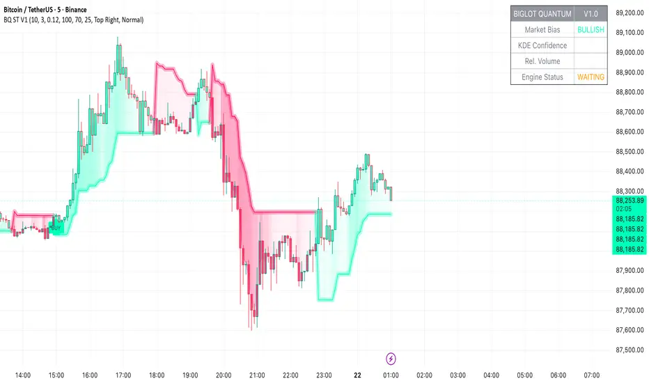
BigLot Quantum SuperTrend V1BigLot Quantum SuperTrend V1 is a trend-following indicator that enhances the traditional SuperTrend by integrating statistical volume analysis.
The script combines an ATR-based SuperTrend engine with Kernel Density Estimation (KDE) applied to relative buy and sell volume. Volume behavior is modeled statistically, allowing the indicator to filter breakout signals and activate only when volume conditions show high probability compared to historical data.
Bullish and bearish signals are generated when price crosses the SuperTrend line and the corresponding volume probability exceeds a user-defined threshold. This approach helps reduce false signals during low-liquidity or sideways market conditions.
The script includes visual trend highlighting, probability-based confidence filtering, and a real-time dashboard displaying trend direction, volume strength, and signal status. It is designed to work across all markets and timeframes without repainting.
SMA MAD Trend [Alpha Extract]A sophisticated trend identification system that combines Simple Moving Average with Mean Absolute Deviation methodology to create adaptive Super Trend-style bands with advanced strength filtering and gradient visualization. Utilizing ADX-based trend strength validation and slope analysis for signal quality enhancement, this indicator delivers institutional-grade trend detection with dynamic ATR-based ribbon visualization and comprehensive strength measurement. The system's dual-filter architecture eliminates false signals during weak or choppy market conditions while maintaining sensitivity to genuine trend establishment and reversal events.
🔶 Advanced SMA-MAD Band Construction
Implements innovative Mean Absolute Deviation calculation around Simple Moving Average baseline to create volatility-adaptive bands with ratcheting logic for trend persistence. The system calculates MAD by measuring absolute price deviations from the mean, then applies configurable multipliers to generate upper and lower bands that adjust to changing market conditions while preventing premature band violations.
// Core SMA-MAD Framework
SMA_Value = ta.sma(close, SMA_Length)
Mean = ta.sma(close, MAD_Length)
Abs_Deviation = abs(close - Mean)
MAD_Value = ta.sma(Abs_Deviation, MAD_Length)
// Adaptive Bands
Upper_Band = SMA_Value + MAD_Factor * MAD_Value
Lower_Band = SMA_Value - MAD_Factor * MAD_Value
🔶 Intelligent Dual-Filter System
Features comprehensive trend validation using ADX strength measurement and slope analysis to eliminate low-conviction signals during ranging or consolidating markets. The system calculates normalized slope strength using ATR scaling and combines with ADX threshold analysis, generating filtered trend states that distinguish genuine trends from temporary price fluctuations.
🔶 Dynamic Trend Strength Engine
Implements sophisticated strength calculation combining slope intensity and ADX readings to produce normalized 0-100% strength scores with gradient colour intensity modulation. The system normalizes slope by minimum threshold and ADX by configurable level, multiplying factors to create composite strength measurement that drives visual feedback intensity across all indicator elements.
🔶 Super Trend-Style Direction Logic
Utilizes classic Super Trend methodology adapted for SMA-MAD bands, where trend direction flips occur on opposite band violations with persistent state maintenance. The system tracks previous band levels with ratcheting behaviour that adjusts bands only when price movement or new calculations warrant changes, preventing oscillation during normal volatility.
🔶 ATR-Based Ribbon Visualization
Provides dynamic ribbon overlay using ATR-scaled width around the trend line with opacity modulation based on trend strength for intuitive conviction assessment. The system creates upper and lower ribbon bounds at configurable ATR multiples, filling the channel with gradient-adjusted transparency that increases during strong trends and fades during weak conditions.
🔶 Multi-Dimensional Visual Architecture
Provides complete chart integration through trend line overlay, ATR ribbon fills, candle colouring, background glow, and transition signal labels with configurable visibility toggles. The system enables traders to customize display density from minimal (trend line only) to comprehensive (all visual elements) while maintaining consistent colour scheme and strength-based intensity across components.
🔶 Slope Strength Validation
Calculates ATR-normalized slope over configurable lookback periods to measure trend line momentum and filter sideways price action. The system compares absolute slope against minimum threshold requirements, preventing trend signals when price movement relative to the trend line lacks sufficient directional conviction regardless of band position.
🔶 Signal Generation Framework
Generates trend change signals when filtered direction state transitions from bearish to bullish or vice versa, with label placement and alert integration. The system implements state persistence that maintains previous trend until both ADX and slope filters confirm directional change, reducing whipsaw signals while capturing genuine reversals with minimal lag.
🔶 Performance Optimization Framework
Utilizes efficient calculation methods with optimized variable management and configurable parameters for balance between responsiveness and stability. The system includes intelligent state tracking with NA handling for initial bars and smooth gradient calculations that maintain performance across extended historical periods and real-time updates.
This indicator delivers sophisticated trend identification through Mean Absolute Deviation methodology combined with dual-strength filtering for superior signal quality. Unlike traditional Super Trend indicators that rely solely on ATR bands, the SMA-MAD approach uses statistical deviation measurement while incorporating ADX strength and slope validation to eliminate false signals during choppy conditions. The system's gradient-based visual feedback, ATR ribbon visualization, comprehensive dashboard, and multi-dimensional filtering make it essential for traders seeking reliable trend-following approaches with clear conviction measurement across cryptocurrency, forex, and equity markets. The combination of adaptive bands, strength-based transparency, and intelligent filtering creates an institutional-grade trend system suitable for systematic trading strategies.

Kijun Sen Standard Deviation | QuantLapse SystemsOverview
The Kijun Sen Standard Deviation indicator by QuantLapse Systems is a volatility-aware trend-following framework that combines the structural equilibrium of the Kijun Sen (基準線) with statistically adaptive standard deviation bands.
By anchoring trend detection to market structure and confirming direction through volatility expansion, the indicator delivers a cleaner, more reliable regime classification across varying market conditions.
Rather than reacting to short-term noise, the system focuses on identifying statistically justified trend phases , making it well-suited for disciplined, rule-based trading.
Technical Composition, Calculation, Key Components & Features
📌 Kijun Sen (基準線) – Structural Trend Baseline
Calculated as the midpoint between the highest high and lowest low over a user-defined period.
Represents market equilibrium and structural balance rather than short-term momentum.
Naturally adapts to expanding and contracting price ranges.
Provides a stable baseline for regime detection and volatility validation.
Acts as the anchor for deviation bands and persistent trend-state logic.
Unlike fast or reactive moving averages, the Kijun Sen emphasizes price structure and equilibrium , making it especially effective for higher-quality trend confirmation.
📌 Volatility Adjustment – Standard Deviation Bands
Standard deviation is calculated over a configurable lookback to measure current price dispersion.
Upper and lower envelopes are formed by applying a deviation multiplier to the Kijun Sen.
Band width expands during volatility surges and contracts during consolidation.
Creates proportional, volatility-aware thresholds instead of static offsets.
Visually represents market energy through expanding and compressing channels.
These adaptive bands ensure that trend signals only occur when volatility supports directional movement.
📌 Trend Signal & Regime Calculation
Bullish Trend is confirmed when price closes above the upper deviation band.
Bearish Trend is confirmed when price closes below the lower deviation band.
Once established, the trend state persists until an opposing volatility break occurs.
This persistence reduces whipsaws and improves regime stability.
Trend state is reinforced with color-coded lines, envelopes, and background shading.
This volatility-confirmed persistence model is visible in the chart, where trends remain intact through minor pullbacks and only flip on decisive expansion.
How It Works in Trading
✅ Volatility-Confirmed Trend Detection – Requires expansion beyond deviation bands.
✅ Noise Suppression – Filters low-energy price movement within volatility envelopes.
✅ Regime Persistence – Maintains trend state until statistical invalidation.
✅ Immediate Visual Context – Direction, strength, and transitions are clear at a glance.
Visual Representation
Trend signals are displayed directly on price using both line and background context:
🟢 Green / Teal Kijun & Envelope → Confirmed bullish regime.
🔴 Red / Pink Kijun & Envelope → Confirmed bearish regime.
Semi-transparent band fill visualizes volatility expansion and compression.
Buy and Sell labels appear only on confirmed regime transitions.
The lower panel includes:
Strategy equity curve based on trend exposure.
Buy & Hold equity for performance comparison.
Background regime shading synchronized with trend state.
Features and User Inputs
The Kijun Sen Standard Deviation framework offers a focused yet powerful set of configurable inputs:
Kijun Sen Length – Controls structural trend sensitivity.
Standard Deviation Controls – Adjust lookback length and multiplier for regime strictness.
Backtesting & Date Filters – Define evaluation periods and starting conditions.
Display Options – Toggle labels, equity curves, and background shading.
Color Customization – Fully configurable buy/sell colors for trends and equity curves.
These controls allow users to balance responsiveness, stability, and clarity without overfitting.
Practical Applications
The Kijun Sen Standard Deviation indicator is designed for traders who prioritize structure, volatility confirmation, and regime awareness.
Primary Trend Filtering – Identify and stay aligned with dominant market direction.
Volatility-Aware Trend Following – Participate only when price expansion confirms intent.
Risk-Managed Exposure – Avoid chop during compression and transitional phases.
Systematic Strategy Development – Use as a regime engine or higher-timeframe filter.
Performance Evaluation – Compare trend-following equity against buy-and-hold benchmarks.
This framework bridges classical Ichimoku structure with modern statistical validation.
Conclusion
The Kijun Sen Standard Deviation indicator by QuantLapse Systems represents a refined evolution of Ichimoku-based trend analysis.
By integrating the structural equilibrium of the Kijun Sen with adaptive standard deviation confirmation, the system delivers clearer regime classification, reduced noise, and more reliable trend participation.
Rather than attempting to predict price, it focuses on confirming when trends are statistically justified .
Who should use Kijun Sen Standard Deviation:
📊 Trend-Following Traders – Stay aligned with dominant market structure.
⚡ Momentum & Swing Traders – Enter only on volatility-backed expansions.
🤖 Systematic & Algorithmic Traders – Ideal as a regime filter or trend-state engine.
Past performance is not indicative of future results.
Disclaimer: All trading involves risk, and no indicator can guarantee profitability.
Strategic Advice: Always backtest thoroughly, optimize parameters responsibly, and align settings with your timeframe, asset class, and risk tolerance before live deployment.

Filtered TEMA CrossoverFiltered Dual TEMA Crossover
This indicator is a trend-following tool based on the classic Dual Triple Exponential Moving Average (TEMA) Crossover strategy, enhanced with two robust filters: the Chop Index and the Average Directional Index (ADX).
The TEMA is known for its low lag and high responsiveness, making the crossover an effective signal for trend reversals. However, trading TEMA crossovers during sideways, choppy markets often leads to false signals. This is where the filters come in.
Key Features
▪️Dual TEMA Crossover: Plots two customizable TEMA lines (Fast and Slow) for clear visualization of the primary trend direction.
▪️Intelligent Signal Filtering: Buy and Sell signals are generated only when the market confirms it is in a trending state, thanks to two integrated filters:
➖Chop Index Filter: Blocks signals when the market is detected as sideways or consolidating (Chop Index reading above a user-defined threshold).
➖ADX Filter: Ensures signals are only taken when the trend strength is sufficient (ADX reading above a user-defined minimum threshold).
▪️Customizable Signals: Full control over the signal shapes (Arrows, Triangles, etc.), colors, text, and size.
How to Use It
Use the Filtered Dual TEMA Crossover to enter positions on trend continuation or reversal while dramatically reducing exposure to low-quality, whipsawing signals common in non-trending environments.
Before the filters:
After the filters:
Minimize Noise. Maximize Clarity. Trade the Trend.

Orderblock Footprints [AlgoAlpha]🟠 OVERVIEW
This script highlights orderblocks and then drills into what actually trades inside them. Zones are created only after an abnormal directional impulse, measured with a z-score on consecutive candle bodies, so the orderblocks are tied to real expansion rather than simple pivots. Once a zone exists, the script overlays lower-timeframe volume footprints inside the candle when price trades back into that zone. The goal is to show not just where an orderblock sits, but whether price is being accepted or absorbed when it is revisited.
🟠 CONCEPTS
Orderblocks are detected after extreme bullish or bearish impulses. The script tracks consecutive body movement up or down, normalizes that distance with a rolling z-score, and only triggers when the move is statistically large. The last opposite candle before that impulse defines the orderblock range. These zones then extend forward until they are either mitigated by price closing through them or they expire by age.
Inside an active zone, the script switches to a lower timeframe and builds a footprint-style profile for each bar. Each candle is split into price rows, counting time-at-price and volume delta. Positive and negative delta are colored separately. Absorption is flagged when opposing delta prints appear in the wick that rejects the zone. In practice: the impulse defines context ; the footprint shows interaction .
🟠 FEATURES
Separate bullish and bearish zones with automatic extension
Volume split inside each zone candle (up vs down volume)
Lower-timeframe footprint with TPO-style rows and delta gradient
Absorption detection using opposing delta in rejection wicks
Alerts for zone creation and absorption events
🟠 USAGE
Setup : Add the script to your chart. It works on any market and timeframe. The lower timeframe for footprints is fixed at 5 minutes, so higher chart timeframes show clearer structure. Use the Z-Score Window to control how strict impulse detection is and Max Box Age to limit how long old zones stay on the chart.
Read the chart : Bullish orderblocks are created after strong upward impulses and are invalidated when price closes below them. Bearish orderblocks are created after strong downward impulses and are invalidated when price closes above them. When price trades inside a zone, footprint rows appear. Green-tinted rows show positive delta; red-tinted rows show negative delta. Absorption labels appear when opposing delta prints into a rejecting wick.
Settings that matter : Increasing the Z-Score Window makes orderblocks rarer but more significant. Disabling Prevent Overlap allows stacked zones if you want to study clustering. Adjusting Rows per bar changes footprint resolution—lower values are cleaner, higher values show more detail but use more objects.

Moving Average Channel Breakout (No Repaint) This indicator creates a channel using two simple moving averages: SMA of highs (upper line) and SMA of lows (lower line).
How it works:
- When a candle closes above the upper channel line, the following candles turn green (bullish trend)
- When a candle closes below the lower channel line, the following candles turn red (bearish trend)
- The trend color remains until a breakout in the opposite direction occurs
Anti-repaint:
This indicator does NOT repaint. The candle color is determined at the open, based on the previous candle's close. Once a candle opens with a color, that color never changes.
Breakout strategy:
- Candle opens green → Long entry signal
- Candle opens red → Short entry signal
The signal and entry moment are perfectly synchronized at the candle open, making it ideal for systematic breakout strategies.

Trend Tracer [AlgoAlpha]🟠 OVERVIEW
This tool builds a two-stage trend model that reacts to structure shifts while also showing how strong or weak the move is. It uses a mid-price band (from the highest high and lowest low over a lookback) and applies two Supertrend passes on top of it. The first pass smoothens the basis. The second pass refines that direction and produces the final trail used for signals. A gradient fill between the two trails uses RSI of price-to-trail distance to show when price is stretched or cooling off. The aim is to give traders a simple way to read trend alignment, pressure, and early turns without guessing.
🟠 CONCEPTS
The script starts with a mid-range basis. This is the average of the rolling highest high and lowest low. It acts as a stable structure reference instead of raw close or typical price. From there, two Supertrend layers are applied:
• The first Supertrend uses a shorter ATR period and lower factor. It reacts faster and sets the main regime.
• The second Supertrend uses a slightly longer ATR and higher factor. It filters noise, waits for confirmed continuation, and generates the signal line.
The interaction between these trails matters. The outer Supertrend provides context by defining the broader regime. The inner Supertrend provides timing by flipping earlier and marking possible shifts. The gradient fill uses RSI of (close − supertrend value) to display when price stretches away from the trail. This shows strength, exhaustion, or compression within the trend.
🟠 FEATURES
Bullish and bearish flip markers placed at recent highs/lows
Rejection signals off the trend tracer line
Alerts for bullish and bearish trend changes
🟠 USAGE
Setup : Add the script to your chart. Timeframe is flexible; lower timeframes show more flips while higher ones give cleaner swings. Adjust Length to change how wide the basis range is. Use the two ATR settings and factors to match the volatility of the market you trade.
Read the chart : When the refined trail (stv_) sits above price the regime is bearish; when below, it is bullish. The wide trail (stv) confirms the larger move. Watch the gradient fill: darker colors appear when price is stretched from the trail and lighter colors appear when the move is weakening. Flip markers ▲ or ▼ highlight the first clean shift of the refined trail.
Settings that matter : Increasing the Main Factor slows main-trend flips and filters chop. Increasing the Signal Factor delays the timing trail but reduces noise. Shortening Length makes the basis more reactive. ATR periods change how sensitive each Supertrend pass is to volatility.
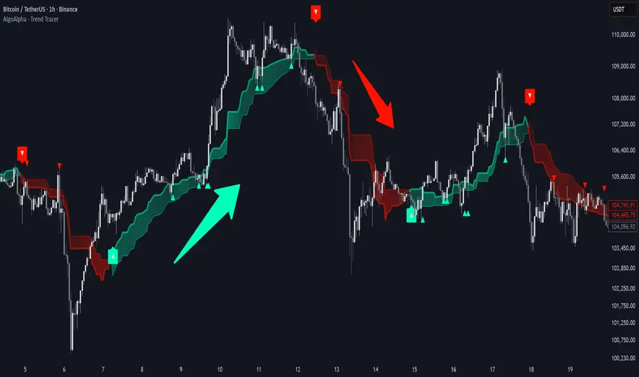
Robrechtian Long-Medium Breakout Trend SystemRobrechtian Long–Medium-Term Breakout Trend System
A professional, rule-based trend-following strategy designed to capture large, sustained price movements using pure price action and breakouts.
This system follows long-established trend-following philosophy: no prediction, no volatility targeting, and no profit targets. Only disciplined entries, position additions, and exits driven entirely by trend structure.
Core Principles
Breakout-driven entries: Initial positions are taken only when price breaks above/below the 80-day Donchian channel, confirming a long–medium-term trend shift.
Short-term confirmation: Breakouts must also exceed the 20-day channel, reducing false positives.
Trend-direction filter: A 50-day moving average slope filter ensures alignment with the broader trend.
Explosive bar filter: Entries avoid excessively large, single-candle expansions (>2.5× ATR(20)) to prevent chasing exhaustion spikes.
Pyramiding into strength: Additional units are added only when price makes fresh 20-day breakouts in the direction of the trend. No scaling out. No adding on dips.
Exit only on trend violation: Positions are closed exclusively when price breaks the opposite 80-day channel. This preserves unlimited upside while enforcing disciplined exits.
Pure trend philosophy: No volatility targeting, no smoothing, no discretionary overrides, no optimization for short-term performance.
Intended Use
This system is designed primarily for diversified futures portfolios, where diversification across dozens of globally liquid markets creates robustness and stability. However, it may also be used on individual assets for educational and analytical purposes.
The system embraces the core trend-following logic:
Small losses, big winners, and unlimited upside when trends persist.
⚠️ WARNINGS / DISCLAIMERS
⚠️ Warning 1 — This strategy is not optimized for single stocks
The Robrechtian Trend System is designed for multi-asset futures portfolios, not single equities.
Performance on individual tickers may vary greatly due to lack of diversification.
⚠️ Warning 2 — Trend following includes substantial drawdowns
Deep drawdowns are a normal and expected feature of all long-term trend-following systems.
The strategy does not attempt to smooth returns or manage volatility.
If you seek steady, low-volatility equity curves, this system is not suitable.
⚠️ Warning 3 — No volatility targeting or risk smoothing
This system intentionally avoids volatility-based position sizing.
Trades may experience larger fluctuations than systems using risk parity or vol targeting.
⚠️ Warning 4 — Not financial advice
This script is for educational and research purposes only.
Past performance does not guarantee future results.
Use at your own risk.
⚠️ Warning 5 — TradingView backtests have known limitations
TradingView does not simulate:
futures contract roll logic
slippage
real bid/ask spreads
liquidity conditions
limit-up/limit-down behavior
Results may vary from live market execution.

5 DMA Entry Plus5 DMA Entry Plus - Multi-Strategy Entry Signal Indicator
Overview:
The 5 DMA Entry Plus is a versatile entry signal indicator that combines multiple proven technical analysis methods to identify potential buy opportunities. This indicator is designed to be highly customizable, allowing traders to toggle between different entry strategies or combine them for confluence-based entries.
Key Features:
1. Multiple Entry Strategy Options:
Default Close Above Entry: Triggers when price closes above the 5-day moving average (with optional HMA filter)
Green Wick Candle Signal: Identifies bullish candles where the wick pierces above key moving averages, indicating rejection of lower prices
5DMA Zero/Upslope Entry: Generates signals when the 5DMA is flat or sloping upward, confirming momentum
HMA Cross Entry: Triggers when price crosses above the Hull Moving Average, a responsive momentum indicator
2. Adaptive HMA Filter:
Toggle the HMA (Hull Moving Average) filter on or off to adjust signal sensitivity. When enabled, price must be above both the 5DMA and 20 HMA for confirmation. When disabled, only the 5DMA is required, generating more frequent signals.
3. Smart Reset Logic:
The indicator includes intelligent reset functionality that prevents signal spam. Once an entry signal is generated, no new signals appear until price closes below the moving average(s), ensuring clean, actionable entries without clutter.
4. Visual Components:
5-Day Moving Average (Blue Line): The primary trend reference
20-Period Hull Moving Average (Orange Line): Fast-responding momentum filter
Buy Signals (Green Labels): Clear "Buy" labels appear below candles when entry conditions are met
Built-in Alerts: Set up custom alerts to be notified when entry signals trigger
Customizable Inputs:
Use HMA Filter: Enable/disable the 20 HMA confirmation requirement
Include Green Wick Candle Signal: Toggle wick-based entry detection
Use 5DMA Zero/Upslope Entry: Enable slope-based entry logic
Use HMA Cross Entry: Enable HMA crossover signals
HMA Length: Adjust the Hull Moving Average period (default: 20)
Best Use Cases:
Swing trading on daily and 4-hour timeframes
Identifying pullback entries in uptrends
Combining multiple confirmation signals for high-probability setups
Filtering entries in momentum-based strategies
Strategy Flexibility:
This indicator allows you to use each entry method independently or combine multiple methods for confluence. Test different combinations to find what works best for your trading style and the instruments you trade.
Risk Management Note:
This indicator identifies potential entry points but does not provide exit signals or stop-loss levels. Always use proper risk management and combine with your own exit strategy.
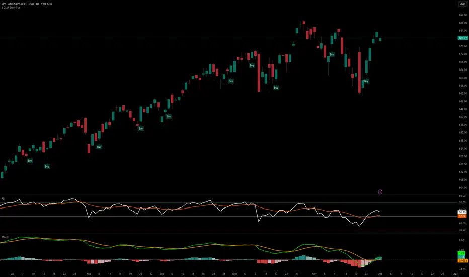
The 'Qualified' POI Scorer [PhenLabs]📊 The “Qualified” POI Scorer (Q-POI)
Version: PineScript™ v6
📌 Description
The “Qualified” POI Scorer helps intermediate traders overcome "analysis paralysis" by filtering Smart Money Concepts (SMC) structures based on their probability. Instead of flooding your chart with every possible Order Block, this script assigns a proprietary “Quality Score” (0-100) to each zone. It analyzes the strength of the displacement, the presence of imbalances (FVG), and liquidity mechanics to determine which zones are worth your attention. It is designed to clean up your charts and enforce discipline by visually fading out low-quality setups.
🚀 Points of Innovation
Dynamic “Glass UI” Transparency that automatically fades weak zones based on their score.
Proprietary Scoring Algorithm (0-100) based on three distinct institutional factors.
Visual Icon System that prints analytical context (💧— 🚀/🐌—🧱) directly on the chart.
Automated Mitigation Tracking that changes the visual state of zones after they are tested.
Displacement Velocity calculation using ATR to verify institutional intent.
🔧 Core Components
Liquidity Sweep Engine: Detects if a pivot point grabbed liquidity from the previous X bars before reversing.
FVG Validator: Checks if the move away from the zone created a valid Fair Value Gap.
Momentum Scorer: Calculates the size of the displacement candle relative to the Average True Range (ATR).
🔥 Key Features
Quality Filtering: Automatically hides or dims zones that score below 50 (user configurable).
State Management: Zones turn grey when mitigated and delete themselves when invalidated.
Visual Scorecard: Displays the exact numeric score on the zone for quick decision-making.
Time-Decay Logic: Keeps the chart clean by managing the lifespan of old zones.
🎨 Visualization
High Score Zones (80-100): Display as bright, semi-solid boxes indicating high probability.
Medium Score Zones (50-79): Display as translucent “glass” boxes.
Low Score Zones (<50): Display as faint “ghost” boxes or are completely hidden.
Rocket Icon (🚀): Indicates high momentum displacement.
Snail Icon (🐌): Indicates low momentum displacement.
Drop Icon (💧): Indicates the zone swept liquidity.
Brick Icon (🧱): Indicates the zone is supported by an FVG.
📖 Usage Guidelines
Swing Structure Length (Default: 5): Controls the sensitivity of the pivot detection; lower numbers create more zones, higher numbers find major swing points.
ATR Length (Default: 14): Determines the lookback period for calculating relative momentum.
Minimum Quality Score (Default: 50): The threshold for which zones are considered “valid” enough to be fully visible.
Bullish/Bearish Colors: Fully customizable colors that adapt their own transparency based on the score.
Show Weak Zones (Default: False): Toggles the visibility of zones that failed the quality check.
✅ Best Use Cases
Filtering noise during high-volatility sessions by focusing only on Score 80+ zones.
Confirming trend continuation entries by looking for the Rocket (🚀) momentum icon.
Avoiding “stale” zones by ignoring any box that has turned grey (Mitigated).
⚠️ Limitations
The indicator is reactive to closed candles and cannot predict news-driven spikes.
Scoring is based on technical structure and does not account for fundamental drivers.
In extremely choppy markets, the ATR filter may produce lower scores due to lack of displacement.
💡 What Makes This Unique
It transforms subjective SMC analysis into an objective, quantifiable score.
The visual hierarchy allows traders to assess chart quality in milliseconds without reading data.
It integrates three separate SMC concepts (Liquidity, Imbalance, Structure) into a single tool.
🔬 How It Works
Step 1: The script identifies a Swing High or Low based on your length input.
Step 2: It looks backward to see if that swing swept liquidity, and looks forward to check for an FVG and displacement.
Step 3: It calculates a weighted score (30pts for Sweep, 30pts for FVG, 40pts for Momentum).
Step 4: It draws the zone with a transparency level designated by the score and appends the relevant icons.
💡 Note:
For the best results, use this indicator on the timeframe you execute trades on (e.g., 15m or 1h). Do not use it to find entries on the 1m chart if your analysis is based on the 4h chart.
