Buscar en scripts para "黄金近20年走势"


20 years old Turtles strategy still work!!original idea from «Way of the Turtle: The Secret Methods that Turned Ordinary People into Legendary Traders» (2007) CURTIS FAITH

DarkPool's Dashboard v2 DarkPool's Dashboard v2 is a comprehensive "Heads-Up Display" (HUD) designed to aggregate critical market data into a single, customizable table overlaid on the price chart. Its primary goal is to declutter the trading workspace by removing the need for multiple separate indicator panes (like RSI, MACD, and Volume below the chart).
The core of the system is a composite Momentum Score, which calculates a value between -100 and +100 based on a weighted average of RSI, MACD, Stochastic, and Rate of Change (ROC). This score drives the main "Signal" output (e.g., STRONG BUY, HOLD, SELL). Additionally, the dashboard integrates a suite of volume analysis tools—including VWAP, OBV, and Volume Delta—alongside volatility and trend filters to provide a complete market health check at a glance.
Key Features
Composite Momentum Score: A unified metric combining four oscillators to gauge the true strength of the move.
Volume Intelligence: Monitors Relative Volume (RVOL), On-Balance Volume (OBV), Volume Delta, and VWAP status.
Trend & Filter Engine: Visualizes trend direction using EMAs and filters signals based on Volatility (ATR) and Trend Strength (EMA Separation).
Dynamic UI: A fully scalable and customizable table that can be positioned anywhere on the screen, with options to toggle specific data rows on or off.
Alert System: Integrated alerts for Volume Spikes, Divergences, and VWAP crossovers.
How to Use
1. Reading the Main Signal The top rows of the dashboard provide the immediate trade bias:
Signal: Displays text such as "STRONG BUY," "BUY," "HOLD," "SELL," or "STRONG SELL."
Momentum Score: A numeric value next to the signal.
> 50: Strong Bullish Momentum.
20 to 50: Moderate Bullish Momentum.
-20 to 20: Neutral / Hold (Chop).
<-20: Bearish Momentum.
2. Volume Analysis
Volume Bar: Visualizes the current volume relative to the Moving Average.
Spike: If the bar turns Orange/Yellow, a Volume Spike (default 2x average) has occurred.
VWAP: Indicates if the price is trading "Above" or "Below" the Volume Weighted Average Price.
Money Flow (MFI): Checks for institutional buying/selling pressure. "OB" means Overbought, "OS" means Oversold.
3. Trend & Volatility
Trend: Shows "UP" or "DOWN" based on Fast/Slow EMA crossovers.
Volatility: Measures the daily range. "HIGH" volatility suggests expansion, while "LOW" suggests compression (potential breakout pending).
4. Filtering Bad Signals The dashboard includes an "ATR Filter" and "Trend Confirmation" logic.
If the market is moving sideways (low ATR), the dashboard may default to "HOLD" or "NEUTRAL" even if oscillators are crossing, preventing false entries during consolidation.
Configuration Settings
Dashboard Settings
Table Position/Width/Scale: adjust the size and location of the table to fit your screen resolution (e.g., increase scale for 4K monitors).
Colors/Transparency: Customize the background and text colors to match your chart theme.
Indicator Settings
Oscillators: Adjust lengths for RSI, MACD, and Stochastic to tune sensitivity.
Volume: Enable or disable specific volume metrics like OBV or Delta.
Display Options: You can toggle specific rows off (e.g., turn off "ADX" or "SMA" if you do not use them) to compact the table.
Filter Settings
Enable ATR Filter: Toggles volatility filtering.
Trend Confirmation Bars: How many bars the trend must persist before the dashboard flips its bias (helps avoid fake-outs).
Disclaimer This indicator is provided for educational and informational purposes only. It does not constitute financial advice, investment recommendations, or a guarantee of future results. Trading cryptocurrencies and financial markets involves a high level of risk. Always perform your own due diligence before making any trading decisions.

Dynamic Equity Allocation Model//@version=6
indicator('Dynamic Equity Allocation Model', shorttitle = 'DEAM', overlay = false, precision = 1, scale = scale.right, max_bars_back = 500)
// DYNAMIC EQUITY ALLOCATION MODEL
// Quantitative framework for dynamic portfolio allocation between stocks and cash.
// Analyzes five dimensions: market regime, risk metrics, valuation, sentiment,
// and macro conditions to generate allocation recommendations (0-100% equity).
//
// Uses real-time data from TradingView including fundamentals (P/E, ROE, ERP),
// volatility indicators (VIX), credit spreads, yield curves, and market structure.
// INPUT PARAMETERS
group1 = 'Model Configuration'
model_type = input.string('Adaptive', 'Allocation Model Type', options = , group = group1, tooltip = 'Conservative: Slower to increase equity, Aggressive: Faster allocation changes, Adaptive: Dynamic based on regime')
use_crisis_detection = input.bool(true, 'Enable Crisis Detection System', group = group1, tooltip = 'Automatic detection and response to crisis conditions')
use_regime_model = input.bool(true, 'Use Market Regime Detection', group = group1, tooltip = 'Identify Bull/Bear/Crisis regimes for dynamic allocation')
group2 = 'Portfolio Risk Management'
target_portfolio_volatility = input.float(12.0, 'Target Portfolio Volatility (%)', minval = 3, maxval = 20, step = 0.5, group = group2, tooltip = 'Target portfolio volatility (Cash reduces volatility: 50% Equity = ~10% vol, 100% Equity = ~20% vol)')
max_portfolio_drawdown = input.float(15.0, 'Maximum Portfolio Drawdown (%)', minval = 5, maxval = 35, step = 2.5, group = group2, tooltip = 'Maximum acceptable PORTFOLIO drawdown (not market drawdown - portfolio with cash has lower drawdown)')
enable_portfolio_risk_scaling = input.bool(true, 'Enable Portfolio Risk Scaling', group = group2, tooltip = 'Scale allocation based on actual portfolio risk characteristics (recommended)')
risk_lookback = input.int(252, 'Risk Calculation Period (Days)', minval = 60, maxval = 504, group = group2, tooltip = 'Period for calculating volatility and risk metrics')
group3 = 'Component Weights (Total = 100%)'
w_regime = input.float(35.0, 'Market Regime Weight (%)', minval = 0, maxval = 100, step = 5, group = group3)
w_risk = input.float(25.0, 'Risk Metrics Weight (%)', minval = 0, maxval = 100, step = 5, group = group3)
w_valuation = input.float(20.0, 'Valuation Weight (%)', minval = 0, maxval = 100, step = 5, group = group3)
w_sentiment = input.float(15.0, 'Sentiment Weight (%)', minval = 0, maxval = 100, step = 5, group = group3)
w_macro = input.float(5.0, 'Macro Weight (%)', minval = 0, maxval = 100, step = 5, group = group3)
group4 = 'Crisis Detection Thresholds'
crisis_vix_threshold = input.float(40, 'Crisis VIX Level', minval = 30, maxval = 80, group = group4, tooltip = 'VIX level indicating crisis conditions (COVID peaked at 82)')
crisis_drawdown_threshold = input.float(15, 'Crisis Drawdown Threshold (%)', minval = 10, maxval = 30, group = group4, tooltip = 'Market drawdown indicating crisis conditions')
crisis_credit_spread = input.float(500, 'Crisis Credit Spread (bps)', minval = 300, maxval = 1000, group = group4, tooltip = 'High yield spread indicating crisis conditions')
group5 = 'Display Settings'
show_components = input.bool(false, 'Show Component Breakdown', group = group5, tooltip = 'Display individual component analysis lines')
show_regime_background = input.bool(true, 'Show Dynamic Background', group = group5, tooltip = 'Color background based on allocation signals')
show_reference_lines = input.bool(false, 'Show Reference Lines', group = group5, tooltip = 'Display allocation percentage reference lines')
show_dashboard = input.bool(true, 'Show Analytics Dashboard', group = group5, tooltip = 'Display comprehensive analytics table')
show_confidence_bands = input.bool(false, 'Show Confidence Bands', group = group5, tooltip = 'Display uncertainty quantification bands')
smoothing_period = input.int(3, 'Smoothing Period', minval = 1, maxval = 10, group = group5, tooltip = 'Smoothing to reduce allocation noise')
background_intensity = input.int(95, 'Background Intensity (%)', minval = 90, maxval = 99, group = group5, tooltip = 'Higher values = more transparent background')
// Styling Options
color_scheme = input.string('EdgeTools', 'Color Theme', options = , group = 'Appearance', tooltip = 'Professional color themes')
use_dark_mode = input.bool(true, 'Optimize for Dark Theme', group = 'Appearance')
main_line_width = input.int(3, 'Main Line Width', minval = 1, maxval = 5, group = 'Appearance')
// DATA RETRIEVAL
// Market Data
sp500 = request.security('SPY', timeframe.period, close)
sp500_high = request.security('SPY', timeframe.period, high)
sp500_low = request.security('SPY', timeframe.period, low)
sp500_volume = request.security('SPY', timeframe.period, volume)
// Volatility Indicators
vix = request.security('VIX', timeframe.period, close)
vix9d = request.security('VIX9D', timeframe.period, close)
vxn = request.security('VXN', timeframe.period, close)
// Fixed Income and Credit
us2y = request.security('US02Y', timeframe.period, close)
us10y = request.security('US10Y', timeframe.period, close)
us3m = request.security('US03MY', timeframe.period, close)
hyg = request.security('HYG', timeframe.period, close)
lqd = request.security('LQD', timeframe.period, close)
tlt = request.security('TLT', timeframe.period, close)
// Safe Haven Assets
gold = request.security('GLD', timeframe.period, close)
usd = request.security('DXY', timeframe.period, close)
yen = request.security('JPYUSD', timeframe.period, close)
// Financial data with fallback values
get_financial_data(symbol, fin_id, period, fallback) =>
data = request.financial(symbol, fin_id, period, ignore_invalid_symbol = true)
na(data) ? fallback : data
// SPY fundamental metrics
spy_earnings_per_share = get_financial_data('AMEX:SPY', 'EARNINGS_PER_SHARE_BASIC', 'TTM', 20.0)
spy_operating_earnings_yield = get_financial_data('AMEX:SPY', 'OPERATING_EARNINGS_YIELD', 'FY', 4.5)
spy_dividend_yield = get_financial_data('AMEX:SPY', 'DIVIDENDS_YIELD', 'FY', 1.8)
spy_buyback_yield = get_financial_data('AMEX:SPY', 'BUYBACK_YIELD', 'FY', 2.0)
spy_net_margin = get_financial_data('AMEX:SPY', 'NET_MARGIN', 'TTM', 12.0)
spy_debt_to_equity = get_financial_data('AMEX:SPY', 'DEBT_TO_EQUITY', 'FY', 0.5)
spy_return_on_equity = get_financial_data('AMEX:SPY', 'RETURN_ON_EQUITY', 'FY', 15.0)
spy_free_cash_flow = get_financial_data('AMEX:SPY', 'FREE_CASH_FLOW', 'TTM', 100000000)
spy_ebitda = get_financial_data('AMEX:SPY', 'EBITDA', 'TTM', 200000000)
spy_pe_forward = get_financial_data('AMEX:SPY', 'PRICE_EARNINGS_FORWARD', 'FY', 18.0)
spy_total_debt = get_financial_data('AMEX:SPY', 'TOTAL_DEBT', 'FY', 500000000)
spy_total_equity = get_financial_data('AMEX:SPY', 'TOTAL_EQUITY', 'FY', 1000000000)
spy_enterprise_value = get_financial_data('AMEX:SPY', 'ENTERPRISE_VALUE', 'FY', 30000000000)
spy_revenue_growth = get_financial_data('AMEX:SPY', 'REVENUE_ONE_YEAR_GROWTH', 'TTM', 5.0)
// Market Breadth Indicators
nya = request.security('NYA', timeframe.period, close)
rut = request.security('IWM', timeframe.period, close)
// Sector Performance
xlk = request.security('XLK', timeframe.period, close)
xlu = request.security('XLU', timeframe.period, close)
xlf = request.security('XLF', timeframe.period, close)
// MARKET REGIME DETECTION
// Calculate Market Trend
sma_20 = ta.sma(sp500, 20)
sma_50 = ta.sma(sp500, 50)
sma_200 = ta.sma(sp500, 200)
ema_10 = ta.ema(sp500, 10)
// Market Structure Score
trend_strength = 0.0
trend_strength := trend_strength + (sp500 > sma_20 ? 1 : -1)
trend_strength := trend_strength + (sp500 > sma_50 ? 1 : -1)
trend_strength := trend_strength + (sp500 > sma_200 ? 2 : -2)
trend_strength := trend_strength + (sma_50 > sma_200 ? 2 : -2)
// Volatility Regime
returns = math.log(sp500 / sp500 )
realized_vol_20d = ta.stdev(returns, 20) * math.sqrt(252) * 100
realized_vol_60d = ta.stdev(returns, 60) * math.sqrt(252) * 100
ewma_vol = ta.ema(math.pow(returns, 2), 20)
realized_vol = math.sqrt(ewma_vol * 252) * 100
vol_premium = vix - realized_vol
// Drawdown Calculation
running_max = ta.highest(sp500, risk_lookback)
current_drawdown = (running_max - sp500) / running_max * 100
// Regime Score
regime_score = 0.0
// Trend Component (40%)
if trend_strength >= 4
regime_score := regime_score + 40
regime_score
else if trend_strength >= 2
regime_score := regime_score + 30
regime_score
else if trend_strength >= 0
regime_score := regime_score + 20
regime_score
else if trend_strength >= -2
regime_score := regime_score + 10
regime_score
else
regime_score := regime_score + 0
regime_score
// Volatility Component (30%)
if vix < 15
regime_score := regime_score + 30
regime_score
else if vix < 20
regime_score := regime_score + 25
regime_score
else if vix < 25
regime_score := regime_score + 15
regime_score
else if vix < 35
regime_score := regime_score + 5
regime_score
else
regime_score := regime_score + 0
regime_score
// Drawdown Component (30%)
if current_drawdown < 3
regime_score := regime_score + 30
regime_score
else if current_drawdown < 7
regime_score := regime_score + 20
regime_score
else if current_drawdown < 12
regime_score := regime_score + 10
regime_score
else if current_drawdown < 20
regime_score := regime_score + 5
regime_score
else
regime_score := regime_score + 0
regime_score
// Classify Regime
market_regime = regime_score >= 80 ? 'Strong Bull' : regime_score >= 60 ? 'Bull Market' : regime_score >= 40 ? 'Neutral' : regime_score >= 20 ? 'Correction' : regime_score >= 10 ? 'Bear Market' : 'Crisis'
// RISK-BASED ALLOCATION
// Calculate Market Risk
parkinson_hl = math.log(sp500_high / sp500_low)
parkinson_vol = parkinson_hl / (2 * math.sqrt(math.log(2))) * math.sqrt(252) * 100
garman_klass_vol = math.sqrt((0.5 * math.pow(math.log(sp500_high / sp500_low), 2) - (2 * math.log(2) - 1) * math.pow(math.log(sp500 / sp500 ), 2)) * 252) * 100
market_volatility_20d = math.max(ta.stdev(returns, 20) * math.sqrt(252) * 100, parkinson_vol)
market_volatility_60d = ta.stdev(returns, 60) * math.sqrt(252) * 100
market_drawdown = current_drawdown
// Initialize risk allocation
risk_allocation = 50.0
if enable_portfolio_risk_scaling
// Volatility-based allocation
vol_based_allocation = target_portfolio_volatility / math.max(market_volatility_20d, 5.0) * 100
vol_based_allocation := math.max(0, math.min(100, vol_based_allocation))
// Drawdown-based allocation
dd_based_allocation = 100.0
if market_drawdown > 1.0
dd_based_allocation := max_portfolio_drawdown / market_drawdown * 100
dd_based_allocation := math.max(0, math.min(100, dd_based_allocation))
dd_based_allocation
// Combine (conservative)
risk_allocation := math.min(vol_based_allocation, dd_based_allocation)
// Dynamic adjustment
current_equity_estimate = 50.0
estimated_portfolio_vol = current_equity_estimate / 100 * market_volatility_20d
estimated_portfolio_dd = current_equity_estimate / 100 * market_drawdown
vol_utilization = estimated_portfolio_vol / target_portfolio_volatility
dd_utilization = estimated_portfolio_dd / max_portfolio_drawdown
risk_utilization = math.max(vol_utilization, dd_utilization)
risk_adjustment_factor = 1.0
if risk_utilization > 1.0
risk_adjustment_factor := math.exp(-0.5 * (risk_utilization - 1.0))
risk_adjustment_factor := math.max(0.5, risk_adjustment_factor)
risk_adjustment_factor
else if risk_utilization < 0.9
risk_adjustment_factor := 1.0 + 0.2 * math.log(1.0 / risk_utilization)
risk_adjustment_factor := math.min(1.3, risk_adjustment_factor)
risk_adjustment_factor
risk_allocation := risk_allocation * risk_adjustment_factor
risk_allocation
else
vol_scalar = target_portfolio_volatility / math.max(market_volatility_20d, 10)
vol_scalar := math.min(1.5, math.max(0.2, vol_scalar))
drawdown_penalty = 0.0
if current_drawdown > max_portfolio_drawdown
drawdown_penalty := (current_drawdown - max_portfolio_drawdown) / max_portfolio_drawdown
drawdown_penalty := math.min(1.0, drawdown_penalty)
drawdown_penalty
risk_allocation := 100 * vol_scalar * (1 - drawdown_penalty)
risk_allocation
risk_allocation := math.max(0, math.min(100, risk_allocation))
// VALUATION ANALYSIS
// Valuation Metrics
actual_pe_ratio = spy_earnings_per_share > 0 ? sp500 / spy_earnings_per_share : spy_pe_forward
actual_earnings_yield = nz(spy_operating_earnings_yield, 0) > 0 ? spy_operating_earnings_yield : 100 / actual_pe_ratio
total_shareholder_yield = spy_dividend_yield + spy_buyback_yield
// Equity Risk Premium (multi-method calculation)
method1_erp = actual_earnings_yield - us10y
method2_erp = actual_earnings_yield + spy_buyback_yield - us10y
payout_ratio = spy_dividend_yield > 0 and actual_earnings_yield > 0 ? spy_dividend_yield / actual_earnings_yield : 0.4
sustainable_growth = spy_return_on_equity * (1 - payout_ratio) / 100
method3_erp = spy_dividend_yield + sustainable_growth * 100 - us10y
implied_growth = spy_revenue_growth * 0.7
method4_erp = total_shareholder_yield + implied_growth - us10y
equity_risk_premium = method1_erp * 0.35 + method2_erp * 0.30 + method3_erp * 0.20 + method4_erp * 0.15
ev_ebitda_ratio = spy_enterprise_value > 0 and spy_ebitda > 0 ? spy_enterprise_value / spy_ebitda : 15.0
debt_equity_health = spy_debt_to_equity < 1.0 ? 1.2 : spy_debt_to_equity < 2.0 ? 1.0 : 0.8
// Valuation Score
base_valuation_score = 50.0
if equity_risk_premium > 4
base_valuation_score := 95
base_valuation_score
else if equity_risk_premium > 3
base_valuation_score := 85
base_valuation_score
else if equity_risk_premium > 2
base_valuation_score := 70
base_valuation_score
else if equity_risk_premium > 1
base_valuation_score := 55
base_valuation_score
else if equity_risk_premium > 0
base_valuation_score := 40
base_valuation_score
else if equity_risk_premium > -1
base_valuation_score := 25
base_valuation_score
else
base_valuation_score := 10
base_valuation_score
growth_adjustment = spy_revenue_growth > 10 ? 10 : spy_revenue_growth > 5 ? 5 : 0
margin_adjustment = spy_net_margin > 15 ? 5 : spy_net_margin < 8 ? -5 : 0
roe_adjustment = spy_return_on_equity > 20 ? 5 : spy_return_on_equity < 10 ? -5 : 0
valuation_score = base_valuation_score + growth_adjustment + margin_adjustment + roe_adjustment
valuation_score := math.max(0, math.min(100, valuation_score * debt_equity_health))
// SENTIMENT ANALYSIS
// VIX Term Structure
vix_term_structure = vix9d > 0 ? vix / vix9d : 1
backwardation = vix_term_structure > 1.05
steep_backwardation = vix_term_structure > 1.15
// Safe Haven Flows
gold_momentum = ta.roc(gold, 20)
dollar_momentum = ta.roc(usd, 20)
yen_momentum = ta.roc(yen, 20)
treasury_momentum = ta.roc(tlt, 20)
safe_haven_flow = gold_momentum * 0.3 + treasury_momentum * 0.3 + dollar_momentum * 0.25 + yen_momentum * 0.15
// Advanced Sentiment Analysis
vix_percentile = ta.percentrank(vix, 252)
vix_zscore = (vix - ta.sma(vix, 252)) / ta.stdev(vix, 252)
vix_momentum = ta.roc(vix, 5)
vvix_proxy = ta.stdev(vix_momentum, 20) * math.sqrt(252)
risk_reversal_proxy = (vix - realized_vol) / realized_vol
// Sentiment Score
base_sentiment = 50.0
vix_adjustment = 0.0
if vix_zscore < -1.5
vix_adjustment := 40
vix_adjustment
else if vix_zscore < -0.5
vix_adjustment := 20
vix_adjustment
else if vix_zscore < 0.5
vix_adjustment := 0
vix_adjustment
else if vix_zscore < 1.5
vix_adjustment := -20
vix_adjustment
else
vix_adjustment := -40
vix_adjustment
term_structure_adjustment = backwardation ? -15 : steep_backwardation ? -30 : 5
vvix_adjustment = vvix_proxy > 2.0 ? -10 : vvix_proxy < 1.0 ? 10 : 0
sentiment_score = base_sentiment + vix_adjustment + term_structure_adjustment + vvix_adjustment
sentiment_score := math.max(0, math.min(100, sentiment_score))
// MACRO ANALYSIS
// Yield Curve
yield_spread_2_10 = us10y - us2y
yield_spread_3m_10 = us10y - us3m
// Credit Conditions
hyg_return = ta.roc(hyg, 20)
lqd_return = ta.roc(lqd, 20)
tlt_return = ta.roc(tlt, 20)
hyg_duration = 4.0
lqd_duration = 8.0
tlt_duration = 17.0
hyg_log_returns = math.log(hyg / hyg )
lqd_log_returns = math.log(lqd / lqd )
hyg_volatility = ta.stdev(hyg_log_returns, 20) * math.sqrt(252)
lqd_volatility = ta.stdev(lqd_log_returns, 20) * math.sqrt(252)
hyg_yield_proxy = -math.log(hyg / hyg ) * 100
lqd_yield_proxy = -math.log(lqd / lqd ) * 100
tlt_yield = us10y
hyg_spread = (hyg_yield_proxy - tlt_yield) * 100
lqd_spread = (lqd_yield_proxy - tlt_yield) * 100
hyg_distance = (hyg - ta.lowest(hyg, 252)) / (ta.highest(hyg, 252) - ta.lowest(hyg, 252))
lqd_distance = (lqd - ta.lowest(lqd, 252)) / (ta.highest(lqd, 252) - ta.lowest(lqd, 252))
default_risk_proxy = 2.0 - (hyg_distance + lqd_distance)
credit_spread = hyg_spread * 0.5 + (hyg_volatility - lqd_volatility) * 1000 * 0.3 + default_risk_proxy * 200 * 0.2
credit_spread := math.max(50, credit_spread)
credit_market_health = hyg_return > lqd_return ? 1 : -1
flight_to_quality = tlt_return > (hyg_return + lqd_return) / 2
// Macro Score
macro_score = 50.0
yield_curve_score = 0
if yield_spread_2_10 > 1.5 and yield_spread_3m_10 > 2
yield_curve_score := 40
yield_curve_score
else if yield_spread_2_10 > 0.5 and yield_spread_3m_10 > 1
yield_curve_score := 30
yield_curve_score
else if yield_spread_2_10 > 0 and yield_spread_3m_10 > 0
yield_curve_score := 20
yield_curve_score
else if yield_spread_2_10 < 0 or yield_spread_3m_10 < 0
yield_curve_score := 10
yield_curve_score
else
yield_curve_score := 5
yield_curve_score
credit_conditions_score = 0
if credit_spread < 200 and not flight_to_quality
credit_conditions_score := 30
credit_conditions_score
else if credit_spread < 400 and credit_market_health > 0
credit_conditions_score := 20
credit_conditions_score
else if credit_spread < 600
credit_conditions_score := 15
credit_conditions_score
else if credit_spread < 1000
credit_conditions_score := 10
credit_conditions_score
else
credit_conditions_score := 0
credit_conditions_score
financial_stability_score = 0
if spy_debt_to_equity < 0.5 and spy_return_on_equity > 15
financial_stability_score := 20
financial_stability_score
else if spy_debt_to_equity < 1.0 and spy_return_on_equity > 10
financial_stability_score := 15
financial_stability_score
else if spy_debt_to_equity < 1.5
financial_stability_score := 10
financial_stability_score
else
financial_stability_score := 5
financial_stability_score
macro_score := yield_curve_score + credit_conditions_score + financial_stability_score
macro_score := math.max(0, math.min(100, macro_score))
// CRISIS DETECTION
crisis_indicators = 0
if vix > crisis_vix_threshold
crisis_indicators := crisis_indicators + 1
crisis_indicators
if vix > 60
crisis_indicators := crisis_indicators + 2
crisis_indicators
if current_drawdown > crisis_drawdown_threshold
crisis_indicators := crisis_indicators + 1
crisis_indicators
if current_drawdown > 25
crisis_indicators := crisis_indicators + 1
crisis_indicators
if credit_spread > crisis_credit_spread
crisis_indicators := crisis_indicators + 1
crisis_indicators
sp500_roc_5 = ta.roc(sp500, 5)
tlt_roc_5 = ta.roc(tlt, 5)
if sp500_roc_5 < -10 and tlt_roc_5 < -5
crisis_indicators := crisis_indicators + 2
crisis_indicators
volume_spike = sp500_volume > ta.sma(sp500_volume, 20) * 2
sp500_roc_1 = ta.roc(sp500, 1)
if volume_spike and sp500_roc_1 < -3
crisis_indicators := crisis_indicators + 1
crisis_indicators
is_crisis = crisis_indicators >= 3
is_severe_crisis = crisis_indicators >= 5
// FINAL ALLOCATION CALCULATION
// Convert regime to base allocation
regime_allocation = market_regime == 'Strong Bull' ? 100 : market_regime == 'Bull Market' ? 80 : market_regime == 'Neutral' ? 60 : market_regime == 'Correction' ? 40 : market_regime == 'Bear Market' ? 20 : 0
// Normalize weights
total_weight = w_regime + w_risk + w_valuation + w_sentiment + w_macro
w_regime_norm = w_regime / total_weight
w_risk_norm = w_risk / total_weight
w_valuation_norm = w_valuation / total_weight
w_sentiment_norm = w_sentiment / total_weight
w_macro_norm = w_macro / total_weight
// Calculate Weighted Allocation
weighted_allocation = regime_allocation * w_regime_norm + risk_allocation * w_risk_norm + valuation_score * w_valuation_norm + sentiment_score * w_sentiment_norm + macro_score * w_macro_norm
// Apply Crisis Override
if use_crisis_detection
if is_severe_crisis
weighted_allocation := math.min(weighted_allocation, 10)
weighted_allocation
else if is_crisis
weighted_allocation := math.min(weighted_allocation, 25)
weighted_allocation
// Model Type Adjustment
model_adjustment = 0.0
if model_type == 'Conservative'
model_adjustment := -10
model_adjustment
else if model_type == 'Aggressive'
model_adjustment := 10
model_adjustment
else if model_type == 'Adaptive'
recent_return = (sp500 - sp500 ) / sp500 * 100
if recent_return > 5
model_adjustment := 5
model_adjustment
else if recent_return < -5
model_adjustment := -5
model_adjustment
// Apply adjustment and bounds
final_allocation = weighted_allocation + model_adjustment
final_allocation := math.max(0, math.min(100, final_allocation))
// Smooth allocation
smoothed_allocation = ta.sma(final_allocation, smoothing_period)
// Calculate portfolio risk metrics (only for internal alerts)
actual_portfolio_volatility = smoothed_allocation / 100 * market_volatility_20d
actual_portfolio_drawdown = smoothed_allocation / 100 * current_drawdown
// VISUALIZATION
// Color definitions
var color primary_color = #2196F3
var color bullish_color = #4CAF50
var color bearish_color = #FF5252
var color neutral_color = #808080
var color text_color = color.white
var color bg_color = #000000
var color table_bg_color = #1E1E1E
var color header_bg_color = #2D2D2D
switch color_scheme // Apply color scheme
'Gold' =>
primary_color := use_dark_mode ? #FFD700 : #DAA520
bullish_color := use_dark_mode ? #FFA500 : #FF8C00
bearish_color := use_dark_mode ? #FF5252 : #D32F2F
neutral_color := use_dark_mode ? #C0C0C0 : #808080
text_color := use_dark_mode ? color.white : color.black
bg_color := use_dark_mode ? #000000 : #FFFFFF
table_bg_color := use_dark_mode ? #1A1A00 : #FFFEF0
header_bg_color := use_dark_mode ? #2D2600 : #F5F5DC
header_bg_color
'EdgeTools' =>
primary_color := use_dark_mode ? #4682B4 : #1E90FF
bullish_color := use_dark_mode ? #4CAF50 : #388E3C
bearish_color := use_dark_mode ? #FF5252 : #D32F2F
neutral_color := use_dark_mode ? #708090 : #696969
text_color := use_dark_mode ? color.white : color.black
bg_color := use_dark_mode ? #000000 : #FFFFFF
table_bg_color := use_dark_mode ? #0F1419 : #F0F8FF
header_bg_color := use_dark_mode ? #1E2A3A : #E6F3FF
header_bg_color
'Behavioral' =>
primary_color := #808080
bullish_color := #00FF00
bearish_color := #8B0000
neutral_color := #FFBF00
text_color := use_dark_mode ? color.white : color.black
bg_color := use_dark_mode ? #000000 : #FFFFFF
table_bg_color := use_dark_mode ? #1A1A1A : #F8F8F8
header_bg_color := use_dark_mode ? #2D2D2D : #E8E8E8
header_bg_color
'Quant' =>
primary_color := #808080
bullish_color := #FFA500
bearish_color := #8B0000
neutral_color := #4682B4
text_color := use_dark_mode ? color.white : color.black
bg_color := use_dark_mode ? #000000 : #FFFFFF
table_bg_color := use_dark_mode ? #0D0D0D : #FAFAFA
header_bg_color := use_dark_mode ? #1A1A1A : #F0F0F0
header_bg_color
'Ocean' =>
primary_color := use_dark_mode ? #20B2AA : #008B8B
bullish_color := use_dark_mode ? #00CED1 : #4682B4
bearish_color := use_dark_mode ? #FF4500 : #B22222
neutral_color := use_dark_mode ? #87CEEB : #2F4F4F
text_color := use_dark_mode ? #F0F8FF : #191970
bg_color := use_dark_mode ? #001F3F : #F0F8FF
table_bg_color := use_dark_mode ? #001A2E : #E6F7FF
header_bg_color := use_dark_mode ? #002A47 : #CCF2FF
header_bg_color
'Fire' =>
primary_color := use_dark_mode ? #FF6347 : #DC143C
bullish_color := use_dark_mode ? #FFD700 : #FF8C00
bearish_color := use_dark_mode ? #8B0000 : #800000
neutral_color := use_dark_mode ? #FFA500 : #CD853F
text_color := use_dark_mode ? #FFFAF0 : #2F1B14
bg_color := use_dark_mode ? #2F1B14 : #FFFAF0
table_bg_color := use_dark_mode ? #261611 : #FFF8F0
header_bg_color := use_dark_mode ? #3D241A : #FFE4CC
header_bg_color
'Matrix' =>
primary_color := use_dark_mode ? #00FF41 : #006400
bullish_color := use_dark_mode ? #39FF14 : #228B22
bearish_color := use_dark_mode ? #FF073A : #8B0000
neutral_color := use_dark_mode ? #00FFFF : #008B8B
text_color := use_dark_mode ? #C0FF8C : #003300
bg_color := use_dark_mode ? #0D1B0D : #F0FFF0
table_bg_color := use_dark_mode ? #0A1A0A : #E8FFF0
header_bg_color := use_dark_mode ? #112B11 : #CCFFCC
header_bg_color
'Arctic' =>
primary_color := use_dark_mode ? #87CEFA : #4169E1
bullish_color := use_dark_mode ? #00BFFF : #0000CD
bearish_color := use_dark_mode ? #FF1493 : #8B008B
neutral_color := use_dark_mode ? #B0E0E6 : #483D8B
text_color := use_dark_mode ? #F8F8FF : #191970
bg_color := use_dark_mode ? #191970 : #F8F8FF
table_bg_color := use_dark_mode ? #141B47 : #F0F8FF
header_bg_color := use_dark_mode ? #1E2A5C : #E0F0FF
header_bg_color
// Transparency settings
bg_transparency = use_dark_mode ? 85 : 92
zone_transparency = use_dark_mode ? 90 : 95
band_transparency = use_dark_mode ? 70 : 85
table_transparency = use_dark_mode ? 80 : 15
// Allocation color
alloc_color = smoothed_allocation >= 80 ? bullish_color : smoothed_allocation >= 60 ? color.new(bullish_color, 30) : smoothed_allocation >= 40 ? primary_color : smoothed_allocation >= 20 ? color.new(bearish_color, 30) : bearish_color
// Dynamic background
var color dynamic_bg_color = na
if show_regime_background
if smoothed_allocation >= 70
dynamic_bg_color := color.new(bullish_color, background_intensity)
dynamic_bg_color
else if smoothed_allocation <= 30
dynamic_bg_color := color.new(bearish_color, background_intensity)
dynamic_bg_color
else if smoothed_allocation > 60 or smoothed_allocation < 40
dynamic_bg_color := color.new(primary_color, math.min(99, background_intensity + 2))
dynamic_bg_color
bgcolor(dynamic_bg_color, title = 'Allocation Signal Background')
// Plot main allocation line
plot(smoothed_allocation, 'Equity Allocation %', color = alloc_color, linewidth = math.max(1, main_line_width))
// Reference lines (static colors for hline)
hline_bullish_color = color_scheme == 'Gold' ? use_dark_mode ? #FFA500 : #FF8C00 : color_scheme == 'EdgeTools' ? use_dark_mode ? #4CAF50 : #388E3C : color_scheme == 'Behavioral' ? #00FF00 : color_scheme == 'Quant' ? #FFA500 : color_scheme == 'Ocean' ? use_dark_mode ? #00CED1 : #4682B4 : color_scheme == 'Fire' ? use_dark_mode ? #FFD700 : #FF8C00 : color_scheme == 'Matrix' ? use_dark_mode ? #39FF14 : #228B22 : color_scheme == 'Arctic' ? use_dark_mode ? #00BFFF : #0000CD : #4CAF50
hline_bearish_color = color_scheme == 'Gold' ? use_dark_mode ? #FF5252 : #D32F2F : color_scheme == 'EdgeTools' ? use_dark_mode ? #FF5252 : #D32F2F : color_scheme == 'Behavioral' ? #8B0000 : color_scheme == 'Quant' ? #8B0000 : color_scheme == 'Ocean' ? use_dark_mode ? #FF4500 : #B22222 : color_scheme == 'Fire' ? use_dark_mode ? #8B0000 : #800000 : color_scheme == 'Matrix' ? use_dark_mode ? #FF073A : #8B0000 : color_scheme == 'Arctic' ? use_dark_mode ? #FF1493 : #8B008B : #FF5252
hline_primary_color = color_scheme == 'Gold' ? use_dark_mode ? #FFD700 : #DAA520 : color_scheme == 'EdgeTools' ? use_dark_mode ? #4682B4 : #1E90FF : color_scheme == 'Behavioral' ? #808080 : color_scheme == 'Quant' ? #808080 : color_scheme == 'Ocean' ? use_dark_mode ? #20B2AA : #008B8B : color_scheme == 'Fire' ? use_dark_mode ? #FF6347 : #DC143C : color_scheme == 'Matrix' ? use_dark_mode ? #00FF41 : #006400 : color_scheme == 'Arctic' ? use_dark_mode ? #87CEFA : #4169E1 : #2196F3
hline(show_reference_lines ? 100 : na, '100% Equity', color = color.new(hline_bullish_color, 70), linestyle = hline.style_dotted, linewidth = 1)
hline(show_reference_lines ? 80 : na, '80% Equity', color = color.new(hline_bullish_color, 40), linestyle = hline.style_dashed, linewidth = 1)
hline(show_reference_lines ? 60 : na, '60% Equity', color = color.new(hline_bullish_color, 60), linestyle = hline.style_dotted, linewidth = 1)
hline(50, '50% Balanced', color = color.new(hline_primary_color, 50), linestyle = hline.style_solid, linewidth = 2)
hline(show_reference_lines ? 40 : na, '40% Equity', color = color.new(hline_bearish_color, 60), linestyle = hline.style_dotted, linewidth = 1)
hline(show_reference_lines ? 20 : na, '20% Equity', color = color.new(hline_bearish_color, 40), linestyle = hline.style_dashed, linewidth = 1)
hline(show_reference_lines ? 0 : na, '0% Equity', color = color.new(hline_bearish_color, 70), linestyle = hline.style_dotted, linewidth = 1)
// Component plots
plot(show_components ? regime_allocation : na, 'Regime', color = color.new(#4ECDC4, 70), linewidth = 1)
plot(show_components ? risk_allocation : na, 'Risk', color = color.new(#FF6B6B, 70), linewidth = 1)
plot(show_components ? valuation_score : na, 'Valuation', color = color.new(#45B7D1, 70), linewidth = 1)
plot(show_components ? sentiment_score : na, 'Sentiment', color = color.new(#FFD93D, 70), linewidth = 1)
plot(show_components ? macro_score : na, 'Macro', color = color.new(#6BCF7F, 70), linewidth = 1)
// Confidence bands
upper_band = plot(show_confidence_bands ? math.min(100, smoothed_allocation + ta.stdev(smoothed_allocation, 20)) : na, color = color.new(neutral_color, band_transparency), display = display.none, title = 'Upper Band')
lower_band = plot(show_confidence_bands ? math.max(0, smoothed_allocation - ta.stdev(smoothed_allocation, 20)) : na, color = color.new(neutral_color, band_transparency), display = display.none, title = 'Lower Band')
fill(upper_band, lower_band, color = show_confidence_bands ? color.new(neutral_color, zone_transparency) : na, title = 'Uncertainty')
// DASHBOARD
if show_dashboard and barstate.islast
var table dashboard = table.new(position.top_right, 2, 20, border_width = 1, bgcolor = color.new(table_bg_color, table_transparency))
table.clear(dashboard, 0, 0, 1, 19)
// Header
header_color = color.new(header_bg_color, 20)
dashboard_text_color = text_color
table.cell(dashboard, 0, 0, 'DEAM', text_color = dashboard_text_color, bgcolor = header_color, text_size = size.normal)
table.cell(dashboard, 1, 0, model_type, text_color = dashboard_text_color, bgcolor = header_color, text_size = size.normal)
// Core metrics
table.cell(dashboard, 0, 1, 'Equity Allocation', text_color = dashboard_text_color, text_size = size.small)
table.cell(dashboard, 1, 1, str.tostring(smoothed_allocation, '##.#') + '%', text_color = alloc_color, text_size = size.small)
table.cell(dashboard, 0, 2, 'Cash Allocation', text_color = dashboard_text_color, text_size = size.small)
cash_color = 100 - smoothed_allocation > 70 ? bearish_color : primary_color
table.cell(dashboard, 1, 2, str.tostring(100 - smoothed_allocation, '##.#') + '%', text_color = cash_color, text_size = size.small)
// Signal
signal_text = 'NEUTRAL'
signal_color = primary_color
if smoothed_allocation >= 70
signal_text := 'BULLISH'
signal_color := bullish_color
signal_color
else if smoothed_allocation <= 30
signal_text := 'BEARISH'
signal_color := bearish_color
signal_color
table.cell(dashboard, 0, 3, 'Signal', text_color = dashboard_text_color, text_size = size.small)
table.cell(dashboard, 1, 3, signal_text, text_color = signal_color, text_size = size.small)
// Market Regime
table.cell(dashboard, 0, 4, 'Regime', text_color = dashboard_text_color, text_size = size.small)
regime_color_display = market_regime == 'Strong Bull' or market_regime == 'Bull Market' ? bullish_color : market_regime == 'Neutral' ? primary_color : market_regime == 'Crisis' ? bearish_color : bearish_color
table.cell(dashboard, 1, 4, market_regime, text_color = regime_color_display, text_size = size.small)
// VIX
table.cell(dashboard, 0, 5, 'VIX Level', text_color = dashboard_text_color, text_size = size.small)
vix_color_display = vix < 20 ? bullish_color : vix < 30 ? primary_color : bearish_color
table.cell(dashboard, 1, 5, str.tostring(vix, '##.##'), text_color = vix_color_display, text_size = size.small)
// Market Drawdown
table.cell(dashboard, 0, 6, 'Market DD', text_color = dashboard_text_color, text_size = size.small)
market_dd_color = current_drawdown < 5 ? bullish_color : current_drawdown < 10 ? primary_color : bearish_color
table.cell(dashboard, 1, 6, '-' + str.tostring(current_drawdown, '##.#') + '%', text_color = market_dd_color, text_size = size.small)
// Crisis Detection
table.cell(dashboard, 0, 7, 'Crisis Detection', text_color = dashboard_text_color, text_size = size.small)
crisis_text = is_severe_crisis ? 'SEVERE' : is_crisis ? 'CRISIS' : 'Normal'
crisis_display_color = is_severe_crisis or is_crisis ? bearish_color : bullish_color
table.cell(dashboard, 1, 7, crisis_text, text_color = crisis_display_color, text_size = size.small)
// Real Data Section
financial_bg = color.new(primary_color, 85)
table.cell(dashboard, 0, 8, 'REAL DATA', text_color = dashboard_text_color, bgcolor = financial_bg, text_size = size.small)
table.cell(dashboard, 1, 8, 'Live Metrics', text_color = dashboard_text_color, bgcolor = financial_bg, text_size = size.small)
// P/E Ratio
table.cell(dashboard, 0, 9, 'P/E Ratio', text_color = dashboard_text_color, text_size = size.small)
pe_color = actual_pe_ratio < 18 ? bullish_color : actual_pe_ratio < 25 ? primary_color : bearish_color
table.cell(dashboard, 1, 9, str.tostring(actual_pe_ratio, '##.#'), text_color = pe_color, text_size = size.small)
// ERP
table.cell(dashboard, 0, 10, 'ERP', text_color = dashboard_text_color, text_size = size.small)
erp_color = equity_risk_premium > 2 ? bullish_color : equity_risk_premium > 0 ? primary_color : bearish_color
table.cell(dashboard, 1, 10, str.tostring(equity_risk_premium, '##.##') + '%', text_color = erp_color, text_size = size.small)
// ROE
table.cell(dashboard, 0, 11, 'ROE', text_color = dashboard_text_color, text_size = size.small)
roe_color = spy_return_on_equity > 20 ? bullish_color : spy_return_on_equity > 10 ? primary_color : bearish_color
table.cell(dashboard, 1, 11, str.tostring(spy_return_on_equity, '##.#') + '%', text_color = roe_color, text_size = size.small)
// D/E Ratio
table.cell(dashboard, 0, 12, 'D/E Ratio', text_color = dashboard_text_color, text_size = size.small)
de_color = spy_debt_to_equity < 0.5 ? bullish_color : spy_debt_to_equity < 1.0 ? primary_color : bearish_color
table.cell(dashboard, 1, 12, str.tostring(spy_debt_to_equity, '##.##'), text_color = de_color, text_size = size.small)
// Shareholder Yield
table.cell(dashboard, 0, 13, 'Dividend+Buyback', text_color = dashboard_text_color, text_size = size.small)
yield_color = total_shareholder_yield > 4 ? bullish_color : total_shareholder_yield > 2 ? primary_color : bearish_color
table.cell(dashboard, 1, 13, str.tostring(total_shareholder_yield, '##.#') + '%', text_color = yield_color, text_size = size.small)
// Component Scores
component_bg = color.new(neutral_color, 80)
table.cell(dashboard, 0, 14, 'Components', text_color = dashboard_text_color, bgcolor = component_bg, text_size = size.small)
table.cell(dashboard, 1, 14, 'Scores', text_color = dashboard_text_color, bgcolor = component_bg, text_size = size.small)
table.cell(dashboard, 0, 15, 'Regime', text_color = dashboard_text_color, text_size = size.small)
regime_score_color = regime_allocation > 60 ? bullish_color : regime_allocation < 40 ? bearish_color : primary_color
table.cell(dashboard, 1, 15, str.tostring(regime_allocation, '##'), text_color = regime_score_color, text_size = size.small)
table.cell(dashboard, 0, 16, 'Risk', text_color = dashboard_text_color, text_size = size.small)
risk_score_color = risk_allocation > 60 ? bullish_color : risk_allocation < 40 ? bearish_color : primary_color
table.cell(dashboard, 1, 16, str.tostring(risk_allocation, '##'), text_color = risk_score_color, text_size = size.small)
table.cell(dashboard, 0, 17, 'Valuation', text_color = dashboard_text_color, text_size = size.small)
val_score_color = valuation_score > 60 ? bullish_color : valuation_score < 40 ? bearish_color : primary_color
table.cell(dashboard, 1, 17, str.tostring(valuation_score, '##'), text_color = val_score_color, text_size = size.small)
table.cell(dashboard, 0, 18, 'Sentiment', text_color = dashboard_text_color, text_size = size.small)
sent_score_color = sentiment_score > 60 ? bullish_color : sentiment_score < 40 ? bearish_color : primary_color
table.cell(dashboard, 1, 18, str.tostring(sentiment_score, '##'), text_color = sent_score_color, text_size = size.small)
table.cell(dashboard, 0, 19, 'Macro', text_color = dashboard_text_color, text_size = size.small)
macro_score_color = macro_score > 60 ? bullish_color : macro_score < 40 ? bearish_color : primary_color
table.cell(dashboard, 1, 19, str.tostring(macro_score, '##'), text_color = macro_score_color, text_size = size.small)
// ALERTS
// Major allocation changes
alertcondition(smoothed_allocation >= 80 and smoothed_allocation < 80, 'High Equity Allocation', 'Equity allocation reached 80% - Bull market conditions')
alertcondition(smoothed_allocation <= 20 and smoothed_allocation > 20, 'Low Equity Allocation', 'Equity allocation dropped to 20% - Defensive positioning')
// Crisis alerts
alertcondition(is_crisis and not is_crisis , 'CRISIS DETECTED', 'Crisis conditions detected - Reducing equity allocation')
alertcondition(is_severe_crisis and not is_severe_crisis , 'SEVERE CRISIS', 'Severe crisis detected - Maximum defensive positioning')
// Regime changes
regime_changed = market_regime != market_regime
alertcondition(regime_changed, 'Regime Change', 'Market regime has changed')
// Risk management alerts
risk_breach = enable_portfolio_risk_scaling and (actual_portfolio_volatility > target_portfolio_volatility * 1.2 or actual_portfolio_drawdown > max_portfolio_drawdown * 1.2)
alertcondition(risk_breach, 'Risk Breach', 'Portfolio risk exceeds target parameters')
// USAGE
// The indicator displays a recommended equity allocation percentage (0-100%).
// Example: 75% allocation = 75% stocks, 25% cash/bonds.
//
// The model combines market regime analysis (trend, volatility, drawdowns),
// risk management (portfolio-level targeting), valuation metrics (P/E, ERP),
// sentiment indicators (VIX term structure), and macro factors (yield curve,
// credit spreads) into a single allocation signal.
//
// Crisis detection automatically reduces exposure when multiple warning signals
// converge. Alerts available for major allocation shifts and regime changes.
//
// Designed for SPY/S&P 500 portfolio allocation. Adjust component weights and
// risk parameters in settings to match your risk tolerance.
View in Pine

PineConnectorLibrary "PineConnector"
This library is a comprehensive alert webhook text generator for PineConnector. It contains every possible alert syntax variation from the documentation, along with some debugging functions.
To use it, just import the library (eg. "import ZenAndTheArtOfTrading/PineConnector/1 as pc") and use pc.buy(licenseID) to send an alert off to PineConnector - assuming all your webhooks etc are set up correctly.
View the PineConnector documentation for more information on how to send the commands you're looking to send (all of this library's function names match the documentation).
all()
Usage: pc.buy(pc_id, freq=pc.all())
Returns: "all"
once_per_bar()
Usage: pc.buy(pc_id, freq=pc.once_per_bar())
Returns: "once_per_bar"
once_per_bar_close()
Usage: pc.buy(pc_id, freq=pc.once_per_bar_close())
Returns: "once_per_bar_close"
na0(value)
Checks if given value is either 'na' or 0. Useful for streamlining scripts with float user setting inputs which default values to 0 since na is unavailable as a user input default.
Parameters:
value (float) : The value to check
Returns: True if the given value is 0 or na
getDecimals()
Calculates how many decimals are on the quote price of the current market.
Returns: The current decimal places on the market quote price
truncate(number, decimals)
Truncates the given number. Required params: mumber.
Parameters:
number (float) : Number to truncate
decimals (int) : Decimal places to cut down to
Returns: The input number, but as a string truncated to X decimals
getPipSize(multiplier)
Calculates the pip size of the current market.
Parameters:
multiplier (int) : The mintick point multiplier (1 by default, 10 for FX/Crypto/CFD but can be used to override when certain markets require)
Returns: The pip size for the current market
toWhole(number)
Converts pips into whole numbers. Required params: number.
Parameters:
number (float) : The pip number to convert into a whole number
Returns: The converted number
toPips(number)
Converts whole numbers back into pips. Required params: number.
Parameters:
number (float) : The whole number to convert into pips
Returns: The converted number
debug(txt, tooltip, displayLabel)
Prints to console and generates a debug label with the given text. Required params: txt.
Parameters:
txt (string) : Text to display
tooltip (string) : Tooltip to display (optional)
displayLabel (bool) : Turns on/off chart label (default: off)
Returns: Nothing
order(licenseID, command, symbol, parameters, accfilter, comment, secret, freq, debug)
Generates an alert string. Required params: licenseID, command.
Parameters:
licenseID (string) : Your PC license ID
command (string) : Command to send
symbol (string) : The symbol to trigger this order on
parameters (string) : Other optional parameters to include
accfilter (float) : Optional minimum account balance filter
comment (string) : Optional comment (maximum 20 characters)
secret (string) : Optional secret key (must be enabled in dashboard)
freq (string) : Alert frequency. Default = "all", options = "once_per_bar", "once_per_bar_close" and "none"
debug (bool) : Turns on/off debug label
Returns: An alert string with valid PC syntax based on supplied parameters
market_order(licenseID, buy, risk, sl, tp, betrigger, beoffset, spread, trailtrig, traildist, trailstep, atrtimeframe, atrperiod, atrmultiplier, atrshift, atrtrigger, symbol, accfilter, comment, secret, freq, debug)
Generates a market entry alert with relevant syntax commands. Required params: licenseID, buy, risk.
Parameters:
licenseID (string) : Your PC license ID
buy (bool) : true=buy/long, false=sell/short
risk (float) : Risk quantity (according to EA settings)
sl (float) : Stop loss distance in pips or price
tp (float) : Take profit distance in pips or price
betrigger (float) : Breakeven will be activated after the position gains this number of pips
beoffset (float) : Offset from entry price. This is the amount of pips you'd like to protect
spread (float) : Enter the position only if the spread is equal or less than the specified value in pips
trailtrig (float) : Trailing stop-loss will be activated after a trade gains this number of pips
traildist (float) : Distance of the trailing stop-loss from current price
trailstep (float) : Moves trailing stop-loss once price moves to favourable by a specified number of pips
atrtimeframe (int) : ATR Trailing Stop timeframe, only updates once per bar close. Options: 1, 5, 15, 30, 60, 240, 1440
atrperiod (int) : ATR averaging period
atrmultiplier (float) : Multiple of ATR to utilise in the new SL computation, default = 1
atrshift (int) : Relative shift of price information, 0 uses latest candle, 1 uses second last, etc. Default = 0
atrtrigger (int) : Activate the trigger of ATR Trailing after market moves favourably by a number of pips. Default = 0 (instant)
symbol (string) : The symbol to trigger this order on (defaults to current symbol)
accfilter (float) : Optional minimum account balance filter
comment (string) : Optional comment (maximum 20 characters)
secret (string) : Optional secret key (must be enabled in dashboard)
freq (string) : Alert frequency. Default = "all", options = "once_per_bar", "once_per_bar_close" and "none"
debug (bool) : Turns on/off debug label
Returns: A market order alert string with valid PC syntax based on supplied parameters
buy(licenseID, risk, sl, tp, betrigger, beoffset, spread, trailtrig, traildist, trailstep, atrtimeframe, atrperiod, atrmultiplier, atrshift, atrtrigger, symbol, accfilter, comment, secret, freq, debug)
Generates a market buy alert with relevant syntax commands. Required params: licenseID, risk.
Parameters:
licenseID (string) : Your PC license ID
risk (float) : Risk quantity (according to EA settings)
sl (float) : Stop loss distance in pips or price
tp (float) : Take profit distance in pips or price
betrigger (float) : Breakeven will be activated after the position gains this number of pips
beoffset (float) : Offset from entry price. This is the amount of pips you'd like to protect
spread (float) : Enter the position only if the spread is equal or less than the specified value in pips
trailtrig (float) : Trailing stop-loss will be activated after a trade gains this number of pips
traildist (float) : Distance of the trailing stop-loss from current price
trailstep (float) : Moves trailing stop-loss once price moves to favourable by a specified number of pips
atrtimeframe (int) : ATR Trailing Stop timeframe, only updates once per bar close. Options: 1, 5, 15, 30, 60, 240, 1440
atrperiod (int) : ATR averaging period
atrmultiplier (float) : Multiple of ATR to utilise in the new SL computation, default = 1
atrshift (int) : Relative shift of price information, 0 uses latest candle, 1 uses second last, etc. Default = 0
atrtrigger (int) : Activate the trigger of ATR Trailing after market moves favourably by a number of pips. Default = 0 (instant)
symbol (string) : The symbol to trigger this order on (defaults to current symbol)
accfilter (float) : Optional minimum account balance filter
comment (string) : Optional comment (maximum 20 characters)
secret (string) : Optional secret key (must be enabled in dashboard)
freq (string) : Alert frequency. Default = "all", options = "once_per_bar", "once_per_bar_close" and "none"
debug (bool) : Turns on/off debug label
Returns: A market order alert string with valid PC syntax based on supplied parameters
sell(licenseID, risk, sl, tp, betrigger, beoffset, spread, trailtrig, traildist, trailstep, atrtimeframe, atrperiod, atrmultiplier, atrshift, atrtrigger, symbol, accfilter, comment, secret, freq, debug)
Generates a market sell alert with relevant syntax commands. Required params: licenseID, risk.
Parameters:
licenseID (string) : Your PC license ID
risk (float) : Risk quantity (according to EA settings)
sl (float) : Stop loss distance in pips or price
tp (float) : Take profit distance in pips or price
betrigger (float) : Breakeven will be activated after the position gains this number of pips
beoffset (float) : Offset from entry price. This is the amount of pips you'd like to protect
spread (float) : Enter the position only if the spread is equal or less than the specified value in pips
trailtrig (float) : Trailing stop-loss will be activated after a trade gains this number of pips
traildist (float) : Distance of the trailing stop-loss from current price
trailstep (float) : Moves trailing stop-loss once price moves to favourable by a specified number of pips
atrtimeframe (int) : ATR Trailing Stop timeframe, only updates once per bar close. Options: 1, 5, 15, 30, 60, 240, 1440
atrperiod (int) : ATR averaging period
atrmultiplier (float) : Multiple of ATR to utilise in the new SL computation, default = 1
atrshift (int) : Relative shift of price information, 0 uses latest candle, 1 uses second last, etc. Default = 0
atrtrigger (int) : Activate the trigger of ATR Trailing after market moves favourably by a number of pips. Default = 0 (instant)
symbol (string) : The symbol to trigger this order on (defaults to current symbol)
accfilter (float) : Optional minimum account balance filter
comment (string) : Optional comment (maximum 20 characters)
secret (string) : Optional secret key (must be enabled in dashboard)
freq (string) : Alert frequency. Default = "all", options = "once_per_bar", "once_per_bar_close" and "none"
debug (bool) : Turns on/off debug label
Returns: A market order alert string with valid PC syntax based on supplied parameters
closeall(licenseID, comment, secret, freq, debug)
Closes all open trades at market regardless of symbol. Required params: licenseID.
Parameters:
licenseID (string) : Your PC license ID
comment (string) : Optional comment to include (max 20 characters)
secret (string) : Optional secret key (must be enabled in dashboard)
freq (string) : Alert frequency. Default = "all", options = "once_per_bar", "once_per_bar_close" and "none"
debug (bool) : Turns on/off debug label
Returns: The required alert syntax as a string
closealleaoff(licenseID, comment, secret, freq, debug)
Closes all open trades at market regardless of symbol, and turns the EA off. Required params: licenseID.
Parameters:
licenseID (string) : Your PC license ID
comment (string) : Optional comment to include (max 20 characters)
secret (string) : Optional secret key (must be enabled in dashboard)
freq (string) : Alert frequency. Default = "all", options = "once_per_bar", "once_per_bar_close" and "none"
debug (bool) : Turns on/off debug label
Returns: The required alert syntax as a string
closelong(licenseID, symbol, comment, secret, freq, debug)
Closes all long trades at market for the given symbol. Required params: licenseID.
Parameters:
licenseID (string) : Your PC license ID
symbol (string) : Symbol to act on (defaults to current symbol)
comment (string) : Optional comment to include (max 20 characters)
secret (string) : Optional secret key (must be enabled in dashboard)
freq (string) : Alert frequency. Default = "all", options = "once_per_bar", "once_per_bar_close" and "none"
debug (bool) : Turns on/off debug label
Returns: The required alert syntax as a string
closeshort(licenseID, symbol, comment, secret, freq, debug)
Closes all open short trades at market for the given symbol. Required params: licenseID.
Parameters:
licenseID (string) : Your PC license ID
symbol (string) : Symbol to act on (defaults to current symbol)
comment (string) : Optional comment to include (max 20 characters)
secret (string) : Optional secret key (must be enabled in dashboard)
freq (string) : Alert frequency. Default = "all", options = "once_per_bar", "once_per_bar_close" and "none"
debug (bool) : Turns on/off debug label
Returns: The required alert syntax as a string
closelongshort(licenseID, symbol, comment, secret, freq, debug)
Closes all open trades at market for the given symbol. Required params: licenseID.
Parameters:
licenseID (string) : Your PC license ID
symbol (string) : Symbol to act on (defaults to current symbol)
comment (string) : Optional comment to include (max 20 characters)
secret (string) : Optional secret key (must be enabled in dashboard)
freq (string) : Alert frequency. Default = "all", options = "once_per_bar", "once_per_bar_close" and "none"
debug (bool) : Turns on/off debug label
Returns: The required alert syntax as a string
closelongbuy(licenseID, risk, symbol, comment, secret, freq, debug)
Close all long positions and open a new long at market for the given symbol with given risk/contracts. Required params: licenseID.
Parameters:
licenseID (string) : Your PC license ID
risk (float) : Risk or contracts (according to EA settings)
symbol (string) : Symbol to act on (defaults to current symbol)
comment (string) : Optional comment to include (max 20 characters)
secret (string) : Optional secret key (must be enabled in dashboard)
freq (string) : Alert frequency. Default = "all", options = "once_per_bar", "once_per_bar_close" and "none"
debug (bool) : Turns on/off debug label
Returns: The required alert syntax as a string
closeshortsell(licenseID, risk, symbol, comment, secret, freq, debug)
Close all short positions and open a new short at market for the given symbol with given risk/contracts. Required params: licenseID, risk.
Parameters:
licenseID (string) : Your PC license ID
risk (float) : Risk or contracts (according to EA settings)
symbol (string) : Symbol to act on (defaults to current symbol)
comment (string) : Optional comment to include (max 20 characters)
secret (string) : Optional secret key (must be enabled in dashboard)
freq (string) : Alert frequency. Default = "all", options = "once_per_bar", "once_per_bar_close" and "none"
debug (bool) : Turns on/off debug label
Returns: The required alert syntax as a string
newsltplong(licenseID, sl, tp, symbol, accfilter, comment, secret, freq, debug)
Updates the stop loss and/or take profit of any open long trades on the given symbol with the given values. Required params: licenseID, sl and/or tp.
Parameters:
licenseID (string) : Your PC license ID
sl (float) : Stop loss pips or price (according to EA settings)
tp (float) : Take profit pips or price (according to EA settings)
symbol (string) : Symbol to act on (defaults to current symbol)
accfilter (float) : Optional minimum account balance filter
comment (string) : Optional comment to include (max 20 characters)
secret (string) : Optional secret key (must be enabled in dashboard)
freq (string) : Alert frequency. Default = "all", options = "once_per_bar", "once_per_bar_close" and "none"
debug (bool) : Turns on/off debug label
Returns: The required alert syntax as a string
newsltpshort(licenseID, sl, tp, symbol, accfilter, comment, secret, freq, debug)
Updates the stop loss and/or take profit of any open short trades on the given symbol with the given values. Required params: licenseID, sl and/or tp.
Parameters:
licenseID (string) : Your PC license ID
sl (float) : Stop loss pips or price (according to EA settings)
tp (float) : Take profit pips or price (according to EA settings)
symbol (string) : Symbol to act on (defaults to current symbol)
accfilter (float) : Optional minimum account balance filter
comment (string) : Optional comment to include (max 20 characters)
secret (string) : Optional secret key (must be enabled in dashboard)
freq (string) : Alert frequency. Default = "all", options = "once_per_bar", "once_per_bar_close" and "none"
debug (bool) : Turns on/off debug label
Returns: The required alert syntax as a string
closelongpct(licenseID, symbol, comment, secret, freq, debug)
Close a percentage of open long positions (according to EA settings). Required params: licenseID.
Parameters:
licenseID (string) : Your PC license ID
symbol (string) : Symbol to act on (defaults to current symbol)
comment (string) : Optional comment to include (max 20 characters)
secret (string) : Optional secret key (must be enabled in dashboard)
freq (string) : Alert frequency. Default = "all", options = "once_per_bar", "once_per_bar_close" and "none"
debug (bool) : Turns on/off debug label
Returns: The required alert syntax as a string
closeshortpct(licenseID, symbol, comment, secret, freq, debug)
Close a percentage of open short positions (according to EA settings). Required params: licenseID.
Parameters:
licenseID (string) : Your PC license ID
symbol (string) : Symbol to act on (defaults to current symbol)
comment (string) : Optional comment to include (max 20 characters)
secret (string) : Optional secret key (must be enabled in dashboard)
freq (string) : Alert frequency. Default = "all", options = "once_per_bar", "once_per_bar_close" and "none"
debug (bool) : Turns on/off debug label
Returns: The required alert syntax as a string
closelongvol(licenseID, risk, symbol, comment, secret, freq, debug)
Close all open long contracts on the current symbol until the given risk value is remaining. Required params: licenseID, risk.
Parameters:
licenseID (string) : Your PC license ID
risk (float) : The quantity to leave remaining
symbol (string) : Symbol to act on (defaults to current symbol)
comment (string) : Optional comment to include (max 20 characters)
secret (string) : Optional secret key (must be enabled in dashboard)
freq (string) : Alert frequency. Default = "all", options = "once_per_bar", "once_per_bar_close" and "none"
debug (bool) : Turns on/off debug label
Returns: The required alert syntax as a string
closeshortvol(licenseID, risk, symbol, comment, secret, freq, debug)
Close all open short contracts on the current symbol until the given risk value is remaining. Required params: licenseID, risk.
Parameters:
licenseID (string) : Your PC license ID
risk (float) : The quantity to leave remaining
symbol (string) : Symbol to act on (defaults to current symbol)
comment (string) : Optional comment to include (max 20 characters)
secret (string) : Optional secret key (must be enabled in dashboard)
freq (string) : Alert frequency. Default = "all", options = "once_per_bar", "once_per_bar_close" and "none"
debug (bool) : Turns on/off debug label
Returns: The required alert syntax as a string
limit_order(licenseID, buy, price, risk, sl, tp, betrigger, beoffset, spread, trailtrig, traildist, trailstep, atrtimeframe, atrperiod, atrmultiplier, atrshift, atrtrigger, symbol, accfilter, comment, secret, freq, debug)
Generates a limit order alert with relevant syntax commands. Required params: licenseID, buy, price, risk.
Parameters:
licenseID (string) : Your PC license ID
buy (bool) : true=buy/long, false=sell/short
price (float) : Price or pips to set limit order (according to EA settings)
risk (float) : Risk quantity (according to EA settings)
sl (float) : Stop loss distance in pips or price
tp (float) : Take profit distance in pips or price
betrigger (float) : Breakeven will be activated after the position gains this number of pips
beoffset (float) : Offset from entry price. This is the amount of pips you'd like to protect
spread (float) : Enter the position only if the spread is equal or less than the specified value in pips
trailtrig (float) : Trailing stop-loss will be activated after a trade gains this number of pips
traildist (float) : Distance of the trailing stop-loss from current price
trailstep (float) : Moves trailing stop-loss once price moves to favourable by a specified number of pips
atrtimeframe (int) : ATR Trailing Stop timeframe, only updates once per bar close. Options: 1, 5, 15, 30, 60, 240, 1440
atrperiod (int) : ATR averaging period
atrmultiplier (float) : Multiple of ATR to utilise in the new SL computation, default = 1
atrshift (int) : Relative shift of price information, 0 uses latest candle, 1 uses second last, etc. Default = 0
atrtrigger (int) : Activate the trigger of ATR Trailing after market moves favourably by a number of pips. Default = 0 (instant)
symbol (string) : The symbol to trigger this order on (defaults to current symbol)
accfilter (float) : Optional minimum account balance filter
comment (string) : Optional comment (maximum 20 characters)
secret (string) : Optional secret key (must be enabled in dashboard)
freq (string) : Alert frequency. Default = "all", options = "once_per_bar", "once_per_bar_close" and "none"
debug (bool) : Turns on/off debug label
Returns: A limit order alert string with valid PC syntax based on supplied parameters
buylimit(licenseID, price, risk, sl, tp, betrigger, beoffset, spread, trailtrig, traildist, trailstep, atrtimeframe, atrperiod, atrmultiplier, atrshift, atrtrigger, symbol, accfilter, comment, secret, freq, debug)
Generates a buylimit order alert with relevant syntax commands. Required params: licenseID, price, risk.
Parameters:
licenseID (string) : Your PC license ID
price (float) : Price or pips to set limit order (according to EA settings)
risk (float) : Risk quantity (according to EA settings)
sl (float) : Stop loss distance in pips or price
tp (float) : Take profit distance in pips or price
betrigger (float) : Breakeven will be activated after the position gains this number of pips
beoffset (float) : Offset from entry price. This is the amount of pips you'd like to protect
spread (float) : Enter the position only if the spread is equal or less than the specified value in pips
trailtrig (float) : Trailing stop-loss will be activated after a trade gains this number of pips
traildist (float) : Distance of the trailing stop-loss from current price
trailstep (float) : Moves trailing stop-loss once price moves to favourable by a specified number of pips
atrtimeframe (int) : ATR Trailing Stop timeframe, only updates once per bar close. Options: 1, 5, 15, 30, 60, 240, 1440
atrperiod (int) : ATR averaging period
atrmultiplier (float) : Multiple of ATR to utilise in the new SL computation, default = 1
atrshift (int) : Relative shift of price information, 0 uses latest candle, 1 uses second last, etc. Default = 0
atrtrigger (int) : Activate the trigger of ATR Trailing after market moves favourably by a number of pips. Default = 0 (instant)
symbol (string) : The symbol to trigger this order on (defaults to current symbol)
accfilter (float) : Optional minimum account balance filter
comment (string) : Optional comment (maximum 20 characters)
secret (string) : Optional secret key (must be enabled in dashboard)
freq (string) : Alert frequency. Default = "all", options = "once_per_bar", "once_per_bar_close" and "none"
debug (bool) : Turns on/off debug label
Returns: A limit order alert string with valid PC syntax based on supplied parameters
selllimit(licenseID, price, risk, sl, tp, betrigger, beoffset, spread, trailtrig, traildist, trailstep, atrtimeframe, atrperiod, atrmultiplier, atrshift, atrtrigger, symbol, accfilter, comment, secret, freq, debug)
Generates a selllimit order alert with relevant syntax commands. Required params: licenseID, price, risk.
Parameters:
licenseID (string) : Your PC license ID
price (float) : Price or pips to set limit order (according to EA settings)
risk (float) : Risk quantity (according to EA settings)
sl (float) : Stop loss distance in pips or price
tp (float) : Take profit distance in pips or price
betrigger (float) : Breakeven will be activated after the position gains this number of pips
beoffset (float) : Offset from entry price. This is the amount of pips you'd like to protect
spread (float) : Enter the position only if the spread is equal or less than the specified value in pips
trailtrig (float) : Trailing stop-loss will be activated after a trade gains this number of pips
traildist (float) : Distance of the trailing stop-loss from current price
trailstep (float) : Moves trailing stop-loss once price moves to favourable by a specified number of pips
atrtimeframe (int) : ATR Trailing Stop timeframe, only updates once per bar close. Options: 1, 5, 15, 30, 60, 240, 1440
atrperiod (int) : ATR averaging period
atrmultiplier (float) : Multiple of ATR to utilise in the new SL computation, default = 1
atrshift (int) : Relative shift of price information, 0 uses latest candle, 1 uses second last, etc. Default = 0
atrtrigger (int) : Activate the trigger of ATR Trailing after market moves favourably by a number of pips. Default = 0 (instant)
symbol (string) : The symbol to trigger this order on (defaults to current symbol)
accfilter (float) : Optional minimum account balance filter
comment (string) : Optional comment (maximum 20 characters)
secret (string) : Optional secret key (must be enabled in dashboard)
freq (string) : Alert frequency. Default = "all", options = "once_per_bar", "once_per_bar_close" and "none"
debug (bool) : Turns on/off debug label
Returns: A limit order alert string with valid PC syntax based on supplied parameters
stop_order(licenseID, buy, price, risk, sl, tp, betrigger, beoffset, spread, trailtrig, traildist, trailstep, atrtimeframe, atrperiod, atrmultiplier, atrshift, atrtrigger, symbol, accfilter, comment, secret, freq, debug)
Generates a stop order alert with relevant syntax commands. Required params: licenseID, buy, price, risk.
Parameters:
licenseID (string) : Your PC license ID
buy (bool) : true=buy/long, false=sell/short
price (float) : Price or pips to set limit order (according to EA settings)
risk (float) : Risk quantity (according to EA settings)
sl (float) : Stop loss distance in pips or price
tp (float) : Take profit distance in pips or price
betrigger (float) : Breakeven will be activated after the position gains this number of pips
beoffset (float) : Offset from entry price. This is the amount of pips you'd like to protect
spread (float) : Enter the position only if the spread is equal or less than the specified value in pips
trailtrig (float) : Trailing stop-loss will be activated after a trade gains this number of pips
traildist (float) : Distance of the trailing stop-loss from current price
trailstep (float) : Moves trailing stop-loss once price moves to favourable by a specified number of pips
atrtimeframe (int) : ATR Trailing Stop timeframe, only updates once per bar close. Options: 1, 5, 15, 30, 60, 240, 1440
atrperiod (int) : ATR averaging period
atrmultiplier (float) : Multiple of ATR to utilise in the new SL computation, default = 1
atrshift (int) : Relative shift of price information, 0 uses latest candle, 1 uses second last, etc. Default = 0
atrtrigger (int) : Activate the trigger of ATR Trailing after market moves favourably by a number of pips. Default = 0 (instant)
symbol (string) : The symbol to trigger this order on (defaults to current symbol)
accfilter (float) : Optional minimum account balance filter
comment (string) : Optional comment (maximum 20 characters)
secret (string) : Optional secret key (must be enabled in dashboard)
freq (string) : Alert frequency. Default = "all", options = "once_per_bar", "once_per_bar_close" and "none"
debug (bool) : Turns on/off debug label
Returns: A stop order alert string with valid PC syntax based on supplied parameters
buystop(licenseID, price, risk, sl, tp, betrigger, beoffset, spread, trailtrig, traildist, trailstep, atrtimeframe, atrperiod, atrmultiplier, atrshift, atrtrigger, symbol, accfilter, comment, secret, freq, debug)
Generates a buystop order alert with relevant syntax commands. Required params: licenseID, price, risk.
Parameters:
licenseID (string) : Your PC license ID
price (float) : Price or pips to set limit order (according to EA settings)
risk (float) : Risk quantity (according to EA settings)
sl (float) : Stop loss distance in pips or price
tp (float) : Take profit distance in pips or price
betrigger (float) : Breakeven will be activated after the position gains this number of pips
beoffset (float) : Offset from entry price. This is the amount of pips you'd like to protect
spread (float) : Enter the position only if the spread is equal or less than the specified value in pips
trailtrig (float) : Trailing stop-loss will be activated after a trade gains this number of pips
traildist (float) : Distance of the trailing stop-loss from current price
trailstep (float) : Moves trailing stop-loss once price moves to favourable by a specified number of pips
atrtimeframe (int) : ATR Trailing Stop timeframe, only updates once per bar close. Options: 1, 5, 15, 30, 60, 240, 1440
atrperiod (int) : ATR averaging period
atrmultiplier (float) : Multiple of ATR to utilise in the new SL computation, default = 1
atrshift (int) : Relative shift of price information, 0 uses latest candle, 1 uses second last, etc. Default = 0
atrtrigger (int) : Activate the trigger of ATR Trailing after market moves favourably by a number of pips. Default = 0 (instant)
symbol (string) : The symbol to trigger this order on (defaults to current symbol)
accfilter (float) : Optional minimum account balance filter
comment (string) : Optional comment (maximum 20 characters)
secret (string) : Optional secret key (must be enabled in dashboard)
freq (string) : Alert frequency. Default = "all", options = "once_per_bar", "once_per_bar_close" and "none"
debug (bool) : Turns on/off debug label
Returns: A stop order alert string with valid PC syntax based on supplied parameters
sellstop(licenseID, price, risk, sl, tp, betrigger, beoffset, spread, trailtrig, traildist, trailstep, atrtimeframe, atrperiod, atrmultiplier, atrshift, atrtrigger, symbol, accfilter, comment, secret, freq, debug)
Generates a sellstop order alert with relevant syntax commands. Required params: licenseID, price, risk.
Parameters:
licenseID (string) : Your PC license ID
price (float) : Price or pips to set limit order (according to EA settings)
risk (float) : Risk quantity (according to EA settings)
sl (float) : Stop loss distance in pips or price
tp (float) : Take profit distance in pips or price
betrigger (float) : Breakeven will be activated after the position gains this number of pips
beoffset (float) : Offset from entry price. This is the amount of pips you'd like to protect
spread (float) : Enter the position only if the spread is equal or less than the specified value in pips
trailtrig (float) : Trailing stop-loss will be activated after a trade gains this number of pips
traildist (float) : Distance of the trailing stop-loss from current price
trailstep (float) : Moves trailing stop-loss once price moves to favourable by a specified number of pips
atrtimeframe (int) : ATR Trailing Stop timeframe, only updates once per bar close. Options: 1, 5, 15, 30, 60, 240, 1440
atrperiod (int) : ATR averaging period
atrmultiplier (float) : Multiple of ATR to utilise in the new SL computation, default = 1
atrshift (int) : Relative shift of price information, 0 uses latest candle, 1 uses second last, etc. Default = 0
atrtrigger (int) : Activate the trigger of ATR Trailing after market moves favourably by a number of pips. Default = 0 (instant)
symbol (string) : The symbol to trigger this order on (defaults to current symbol)
accfilter (float) : Optional minimum account balance filter
comment (string) : Optional comment (maximum 20 characters)
secret (string) : Optional secret key (must be enabled in dashboard)
freq (string) : Alert frequency. Default = "all", options = "once_per_bar", "once_per_bar_close" and "none"
debug (bool) : Turns on/off debug label
Returns: A stop order alert string with valid PC syntax based on supplied parameters
cancel_neworder(licenseID, order, price, risk, sl, tp, betrigger, beoffset, spread, trailtrig, traildist, trailstep, atrtimeframe, atrperiod, atrmultiplier, atrshift, atrtrigger, symbol, accfilter, comment, secret, freq, debug)
Cancel + place new order template function.
Parameters:
licenseID (string) : Your PC license ID
order (string) : Cancel order type
price (float) : Price or pips to set limit order (according to EA settings)
risk (float) : Risk quantity (according to EA settings)
sl (float) : Stop loss distance in pips or price
tp (float) : Take profit distance in pips or price
betrigger (float) : Breakeven will be activated after the position gains this number of pips
beoffset (float) : Offset from entry price. This is the amount of pips you'd like to protect
spread (float) : Enter the position only if the spread is equal or less than the specified value in pips
trailtrig (float) : Trailing stop-loss will be activated after a trade gains this number of pips
traildist (float) : Distance of the trailing stop-loss from current price
trailstep (float) : Moves trailing stop-loss once price moves to favourable by a specified number of pips
atrtimeframe (int) : ATR Trailing Stop timeframe, only updates once per bar close. Options: 1, 5, 15, 30, 60, 240, 1440
atrperiod (int) : ATR averaging period
atrmultiplier (float) : Multiple of ATR to utilise in the new SL computation, default = 1
atrshift (int) : Relative shift of price information, 0 uses latest candle, 1 uses second last, etc. Default = 0
atrtrigger (int) : Activate the trigger of ATR Trailing after market moves favourably by a number of pips. Default = 0 (instant)
symbol (string) : The symbol to trigger this order on (defaults to current symbol)
accfilter (float) : Optional minimum account balance filter
comment (string) : Optional comment (maximum 20 characters)
secret (string) : Optional secret key (must be enabled in dashboard)
freq (string) : Alert frequency. Default = "all", options = "once_per_bar", "once_per_bar_close" and "none"
debug (bool) : Turns on/off debug label
Returns: A stop order alert string with valid PC syntax based on supplied parameters
cancellongbuystop(licenseID, price, risk, sl, tp, betrigger, beoffset, spread, trailtrig, traildist, trailstep, atrtimeframe, atrperiod, atrmultiplier, atrshift, atrtrigger, symbol, accfilter, comment, secret, freq, debug)
Cancels all long orders with the specified symbol and places a new buystop order. Required params: licenseID, price, risk.
Parameters:
licenseID (string) : Your PC license ID
price (float) : Price or pips to set limit order (according to EA settings)
risk (float) : Risk quantity (according to EA settings)
sl (float) : Stop loss distance in pips or price
tp (float) : Take profit distance in pips or price
betrigger (float) : Breakeven will be activated after the position gains this number of pips
beoffset (float) : Offset from entry price. This is the amount of pips you'd like to protect
spread (float) : Enter the position only if the spread is equal or less than the specified value in pips
trailtrig (float) : Trailing stop-loss will be activated after a trade gains this number of pips
traildist (float) : Distance of the trailing stop-loss from current price
trailstep (float) : Moves trailing stop-loss once price moves to favourable by a specified number of pips
atrtimeframe (int) : ATR Trailing Stop timeframe, only updates once per bar close. Options: 1, 5, 15, 30, 60, 240, 1440
atrperiod (int) : ATR averaging period
atrmultiplier (float) : Multiple of ATR to utilise in the new SL computation, default = 1
atrshift (int) : Relative shift of price information, 0 uses latest candle, 1 uses second last, etc. Default = 0
atrtrigger (int) : Activate the trigger of ATR Trailing after market moves favourably by a number of pips. Default = 0 (instant)
symbol (string) : The symbol to trigger this order on (defaults to current symbol)
accfilter (float) : Optional minimum account balance filter
comment (string) : Optional comment (maximum 20 characters)
secret (string) : Optional secret key (must be enabled in dashboard)
freq (string) : Alert frequency. Default = "all", options = "once_per_bar", "once_per_bar_close" and "none"
debug (bool) : Turns on/off debug label
Returns: A stop order alert string with valid PC syntax based on supplied parameters
cancellongbuylimit(licenseID, price, risk, sl, tp, betrigger, beoffset, spread, trailtrig, traildist, trailstep, atrtimeframe, atrperiod, atrmultiplier, atrshift, atrtrigger, symbol, accfilter, comment, secret, freq, debug)
Cancels all long orders with the specified symbol and places a new buylimit order. Required params: licenseID, price, risk.
Parameters:
licenseID (string) : Your PC license ID
price (float) : Price or pips to set limit order (according to EA settings)
risk (float) : Risk quantity (according to EA settings)
sl (float) : Stop loss distance in pips or price
tp (float) : Take profit distance in pips or price
betrigger (float) : Breakeven will be activated after the position gains this number of pips
beoffset (float) : Offset from entry price. This is the amount of pips you'd like to protect
spread (float) : Enter the position only if the spread is equal or less than the specified value in pips
trailtrig (float) : Trailing stop-loss will be activated after a trade gains this number of pips
traildist (float) : Distance of the trailing stop-loss from current price
trailstep (float) : Moves trailing stop-loss once price moves to favourable by a specified number of pips
atrtimeframe (int) : ATR Trailing Stop timeframe, only updates once per bar close. Options: 1, 5, 15, 30, 60, 240, 1440
atrperiod (int) : ATR averaging period
atrmultiplier (float) : Multiple of ATR to utilise in the new SL computation, default = 1
atrshift (int) : Relative shift of price information, 0 uses latest candle, 1 uses second last, etc. Default = 0
atrtrigger (int) : Activate the trigger of ATR Trailing after market moves favourably by a number of pips. Default = 0 (instant)
symbol (string) : The symbol to trigger this order on (defaults to current symbol)
accfilter (float) : Optional minimum account balance filter
comment (string) : Optional comment (maximum 20 characters)
secret (string) : Optional secret key (must be enabled in dashboard)
freq (string) : Alert frequency. Default = "all", options = "once_per_bar", "once_per_bar_close" and "none"
debug (bool) : Turns on/off debug label
Returns: A stop order alert string with valid PC syntax based on supplied parameters
cancelshortsellstop(licenseID, price, risk, sl, tp, betrigger, beoffset, spread, trailtrig, traildist, trailstep, atrtimeframe, atrperiod, atrmultiplier, atrshift, atrtrigger, symbol, accfilter, comment, secret, freq, debug)
Cancels all short orders with the specified symbol and places a sellstop order. Required params: licenseID, price, risk.
Parameters:
licenseID (string) : Your PC license ID
price (float) : Price or pips to set limit order (according to EA settings)
risk (float) : Risk quantity (according to EA settings)
sl (float) : Stop loss distance in pips or price
tp (float) : Take profit distance in pips or price
betrigger (float) : Breakeven will be activated after the position gains this number of pips
beoffset (float) : Offset from entry price. This is the amount of pips you'd like to protect
spread (float) : Enter the position only if the spread is equal or less than the specified value in pips
trailtrig (float) : Trailing stop-loss will be activated after a trade gains this number of pips
traildist (float) : Distance of the trailing stop-loss from current price
trailstep (float) : Moves trailing stop-loss once price moves to favourable by a specified number of pips
atrtimeframe (int) : ATR Trailing Stop timeframe, only updates once per bar close. Options: 1, 5, 15, 30, 60, 240, 1440
atrperiod (int) : ATR averaging period
atrmultiplier (float) : Multiple of ATR to utilise in the new SL computation, default = 1
atrshift (int) : Relative shift of price information, 0 uses latest candle, 1 uses second last, etc. Default = 0
atrtrigger (int) : Activate the trigger of ATR Trailing after market moves favourably by a number of pips. Default = 0 (instant)
symbol (string) : The symbol to trigger this order on (defaults to current symbol)
accfilter (float) : Optional minimum account balance filter
comment (string) : Optional comment (maximum 20 characters)
secret (string) : Optional secret key (must be enabled in dashboard)
freq (string) : Alert frequency. Default = "all", options = "once_per_bar", "once_per_bar_close" and "none"
debug (bool) : Turns on/off debug label
Returns: A stop order alert string with valid PC syntax based on supplied parameters
cancelshortselllimit(licenseID, price, risk, sl, tp, betrigger, beoffset, spread, trailtrig, traildist, trailstep, atrtimeframe, atrperiod, atrmultiplier, atrshift, atrtrigger, symbol, accfilter, comment, secret, freq, debug)
Cancels all short orders with the specified symbol and places a selllimit order. Required params: licenseID, price, risk.
Parameters:
licenseID (string) : Your PC license ID
price (float) : Price or pips to set limit order (according to EA settings)
risk (float) : Risk quantity (according to EA settings)
sl (float) : Stop loss distance in pips or price
tp (float) : Take profit distance in pips or price
betrigger (float) : Breakeven will be activated after the position gains this number of pips
beoffset (float) : Offset from entry price. This is the amount of pips you'd like to protect
spread (float) : Enter the position only if the spread is equal or less than the specified value in pips
trailtrig (float) : Trailing stop-loss will be activated after a trade gains this number of pips
traildist (float) : Distance of the trailing stop-loss from current price
trailstep (float) : Moves trailing stop-loss once price moves to favourable by a specified number of pips
atrtimeframe (int) : ATR Trailing Stop timeframe, only updates once per bar close. Options: 1, 5, 15, 30, 60, 240, 1440
atrperiod (int) : ATR averaging period
atrmultiplier (float) : Multiple of ATR to utilise in the new SL computation, default = 1
atrshift (int) : Relative shift of price information, 0 uses latest candle, 1 uses second last, etc. Default = 0
atrtrigger (int) : Activate the trigger of ATR Trailing after market moves favourably by a number of pips. Default = 0 (instant)
symbol (string) : The symbol to trigger this order on (defaults to current symbol)
accfilter (float) : Optional minimum account balance filter
comment (string) : Optional comment (maximum 20 characters)
secret (string) : Optional secret key (must be enabled in dashboard)
freq (string) : Alert frequency. Default = "all", options = "once_per_bar", "once_per_bar_close" and "none"
debug (bool) : Turns on/off debug label
Returns: A stop order alert string with valid PC syntax based on supplied parameters
cancellong(licenseID, symbol, accfilter, comment, secret, freq, debug)
Cancels all pending long orders with the specified symbol. Required params: licenseID.
Parameters:
licenseID (string) : Your PC license ID
symbol (string) : Symbol to act on (defaults to current symbol)
accfilter (float) : Optional minimum account balance filter
comment (string) : Optional comment to include (max 20 characters)
secret (string) : Optional secret key (must be enabled in dashboard)
freq (string) : Alert frequency. Default = "all", options = "once_per_bar", "once_per_bar_close" and "none"
debug (bool) : Turns on/off debug label
Returns: A cancel long alert command
cancelshort(licenseID, symbol, accfilter, comment, secret, freq, debug)
Cancels all pending short orders with the specified symbol. Required params: licenseID.
Parameters:
licenseID (string) : Your PC license ID
symbol (string) : Symbol to act on (defaults to current symbol)
accfilter (float) : Optional minimum account balance filter
comment (string) : Optional comment to include (max 20 characters)
secret (string) : Optional secret key (must be enabled in dashboard)
freq (string) : Alert frequency. Default = "all", options = "once_per_bar", "once_per_bar_close" and "none"
debug (bool) : Turns on/off debug label
Returns: A cancel short alert command
newsltpbuystop(licenseID, sl, tp, symbol, accfilter, comment, secret, freq, debug)
Updates the stop loss and/or take profit of any pending buy stop orders on the given symbol. Required params: licenseID, sl and/or tp.
Parameters:
licenseID (string) : Your PC license ID
sl (float) : Stop loss pips or price (according to EA settings)
tp (float) : Take profit pips or price (according to EA settings)
symbol (string) : Symbol to act on (defaults to current symbol)
accfilter (float) : Optional minimum account balance filter
comment (string) : Optional comment to include (max 20 characters)
secret (string) : Optional secret key (must be enabled in dashboard)
freq (string) : Alert frequency. Default = "all", options = "once_per_bar", "once_per_bar_close" and "none"
debug (bool) : Turns on/off debug label
Returns: The required alert syntax as a string
newsltpbuylimit(licenseID, sl, tp, symbol, accfilter, comment, secret, freq, debug)
Updates the stop loss and/or take profit of any pending buy limit orders on the given symbol. Required params: licenseID, sl and/or tp.
Parameters:
licenseID (string) : Your PC license ID
sl (float) : Stop loss pips or price (according to EA settings)
tp (float) : Take profit pips or price (according to EA settings)
symbol (string) : Symbol to act on (defaults to current symbol)
accfilter (float) : Optional minimum account balance filter
comment (string) : Optional comment to include (max 20 characters)
secret (string) : Optional secret key (must be enabled in dashboard)
freq (string) : Alert frequency. Default = "all", options = "once_per_bar", "once_per_bar_close" and "none"
debug (bool) : Turns on/off debug label
Returns: The required alert syntax as a string
newsltpsellstop(licenseID, sl, tp, symbol, accfilter, comment, secret, freq, debug)
Updates the stop loss and/or take profit of any pending sell stop orders on the given symbol. Required params: licenseID, sl and/or tp.
Parameters:
licenseID (string) : Your PC license ID
sl (float) : Stop loss pips or price (according to EA settings)
tp (float) : Take profit pips or price (according to EA settings)
symbol (string) : Symbol to act on (defaults to current symbol)
accfilter (float) : Optional minimum account balance filter
comment (string) : Optional comment to include (max 20 characters)
secret (string) : Optional secret key (must be enabled in dashboard)
freq (string) : Alert frequency. Default = "all", options = "once_per_bar", "once_per_bar_close" and "none"
debug (bool) : Turns on/off debug label
Returns: The required alert syntax as a string
newsltpselllimit(licenseID, sl, tp, symbol, accfilter, comment, secret, freq, debug)
Updates the stop loss and/or take profit of any pending sell limit orders on the given symbol. Required params: licenseID, sl and/or tp.
Parameters:
licenseID (string) : Your PC license ID
sl (float) : Stop loss pips or price (according to EA settings)
tp (float) : Take profit pips or price (according to EA settings)
symbol (string) : Symbol to act on (defaults to current symbol)
accfilter (float) : Optional minimum account balance filter
comment (string) : Optional comment to include (max 20 characters)
secret (string) : Optional secret key (must be enabled in dashboard)
freq (string) : Alert frequency. Default = "all", options = "once_per_bar", "once_per_bar_close" and "none"
debug (bool) : Turns on/off debug label
Returns: The required alert syntax as a string
eaoff(licenseID, secret, freq, debug)
Turns the EA off. Required params: licenseID.
Parameters:
licenseID (string) : Your PC license ID
secret (string) : Optional secret key (must be enabled in dashboard)
freq (string) : Alert frequency. Default = "all", options = "once_per_bar", "once_per_bar_close" and "none"
debug (bool) : Turns on/off debug label
Returns: The required alert syntax as a string
eaon(licenseID, secret, freq, debug)
Turns the EA on. Required params: licenseID.
Parameters:
licenseID (string) : Your PC license ID
secret (string) : Optional secret key (must be enabled in dashboard)
freq (string) : Alert frequency. Default = "all", options = "once_per_bar", "once_per_bar_close" and "none"
debug (bool) : Turns on/off debug label
Returns: The required alert syntax as a string
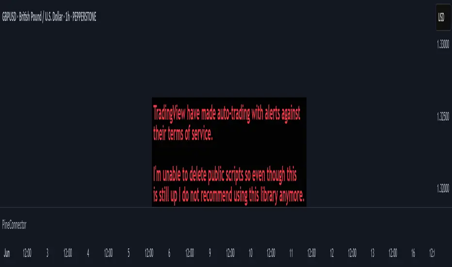
Scout Regiment - KSI# Scout Regiment - KSI Indicator
## English Documentation
### Overview
Scout Regiment - KSI (Key Stochastic Indicators) is a comprehensive momentum oscillator that combines three powerful technical indicators - RSI, CCI, and Williams %R - into a single, unified display. This multi-indicator approach provides traders with diverse perspectives on market momentum, overbought/oversold conditions, and potential reversal points through advanced divergence detection.
### What is KSI?
KSI stands for "Key Stochastic Indicators" - a composite momentum indicator that:
- Displays multiple oscillators normalized to a 0-100 scale
- Uses standardized bands (20/50/80) for consistent interpretation
- Combines RSI for trend, CCI for cycle, and Williams %R for reversal detection
- Provides enhanced divergence detection specifically for RSI
### Key Features
#### 1. **Triple Oscillator System**
**① RSI (Relative Strength Index)** - Primary Indicator
- **Purpose**: Measures momentum and identifies overbought/oversold conditions
- **Default Length**: 22 periods
- **Display**: Blue line (2px)
- **Key Levels**:
- Above 50: Bullish momentum
- Below 50: Bearish momentum
- Above 80: Overbought
- Below 20: Oversold
- **Special Features**:
- Background color indication (green/red)
- Crossover labels at 50 level
- Full divergence detection (4 types)
**② CCI (Commodity Channel Index)** - Dual Period
- **Purpose**: Identifies cyclical trends and extreme conditions
- **Dual Display**:
- CCI(33): Short-term cycle - Green line (1px)
- CCI(77): Medium-term cycle - Orange line (1px)
- **Default Source**: HLC3 (typical price)
- **Normalized Scale**: Mapped from ±100 to 0-100 for consistency
- **Interpretation**:
- Above 80: Strong upward momentum
- Below 20: Strong downward momentum
- 50 level: Neutral
- Divergence between periods: Trend change warning
**③ Williams %R** - Optional
- **Purpose**: Identifies overbought/oversold extremes
- **Default Length**: 28 periods
- **Display**: Magenta line (2px)
- **Scale**: Inverted and normalized to 0-100
- **Best For**: Short-term reversal signals
- **Default**: Disabled (enable when needed for extra confirmation)
#### 2. **Standardized Band System**
**Three-Level Structure:**
- **Upper Band (80)**: Overbought zone
- Strong momentum area
- Watch for reversal signals
- Divergences here are most reliable
- **Middle Line (50)**: Equilibrium
- Separates bullish/bearish zones
- Crossovers indicate momentum shifts
- Key decision level
- **Lower Band (20)**: Oversold zone
- Weak momentum area
- Look for bounce signals
- Divergences here signal potential reversals
**Band Fill**: Dark background between 20-80 for visual clarity
#### 3. **RSI Visual Enhancements**
**Background Color Indication**
- Green background: RSI above 50 (bullish bias)
- Red background: RSI below 50 (bearish bias)
- Optional display for cleaner charts
- Helps identify overall momentum direction
**Crossover Labels**
- "突破" (Breakout): RSI crosses above 50
- "跌破" (Breakdown): RSI crosses below 50
- Marks momentum shift points
- Can be toggled on/off
#### 4. **Advanced RSI Divergence Detection**
The indicator includes comprehensive divergence detection for RSI only (most reliable oscillator):
**Regular Bullish Divergence (Yellow)**
- **Price**: Lower lows
- **RSI**: Higher lows
- **Signal**: Potential upward reversal
- **Label**: "涨" (Up)
- **Most Common**: Near oversold levels (below 30)
**Regular Bearish Divergence (Blue)**
- **Price**: Higher highs
- **RSI**: Lower highs
- **Signal**: Potential downward reversal
- **Label**: "跌" (Down)
- **Most Common**: Near overbought levels (above 70)
**Hidden Bullish Divergence (Light Yellow)**
- **Price**: Higher lows
- **RSI**: Lower lows
- **Signal**: Uptrend continuation
- **Label**: "隐涨" (Hidden Up)
- **Use**: Add to existing longs
**Hidden Bearish Divergence (Light Blue)**
- **Price**: Lower highs
- **RSI**: Higher highs
- **Signal**: Downtrend continuation
- **Label**: "隐跌" (Hidden Down)
- **Use**: Add to existing shorts
**Divergence Parameters** (Fully Customizable):
- **Right Lookback**: Bars to right of pivot (default: 5)
- **Left Lookback**: Bars to left of pivot (default: 5)
- **Max Range**: Maximum bars between pivots (default: 60)
- **Min Range**: Minimum bars between pivots (default: 5)
### Configuration Settings
#### KSI Display Settings
- **Show RSI**: Toggle RSI indicator
- **Show CCI**: Toggle both CCI lines
- **Show Williams %R**: Toggle Williams %R (optional)
#### RSI Settings
- **RSI Length**: Period for calculation (default: 22)
- **Data Source**: Price source (default: close)
- **Show Background**: Toggle green/red background
- **Show Cross Labels**: Toggle 50-level crossover labels
#### RSI Divergence Settings
- **Right Lookback**: Pivot detection right side
- **Left Lookback**: Pivot detection left side
- **Max Range**: Maximum lookback distance
- **Min Range**: Minimum lookback distance
- **Show Regular Divergence**: Enable regular divergence lines
- **Show Regular Labels**: Enable regular divergence labels
- **Show Hidden Divergence**: Enable hidden divergence lines
- **Show Hidden Labels**: Enable hidden divergence labels
#### CCI Settings
- **CCI Length**: Short-term period (default: 33)
- **CCI Mid Length**: Medium-term period (default: 77)
- **Data Source**: Price calculation (default: HLC3)
- **Show CCI(33)**: Toggle short-term CCI
- **Show CCI(77)**: Toggle medium-term CCI
#### Williams %R Settings
- **Length**: Calculation period (default: 28)
- **Data Source**: Price source (default: close)
### How to Use
#### For Basic Momentum Trading
1. **Enable RSI Only** (primary indicator)
- Focus on 50-level crossovers
- Enable crossover labels for signals
2. **Identify Momentum Direction**
- RSI > 50 = Bullish momentum
- RSI < 50 = Bearish momentum
- Background color confirms direction
3. **Look for Extremes**
- RSI > 80 = Overbought (consider selling)
- RSI < 20 = Oversold (consider buying)
4. **Trade Setup**
- Enter long when RSI crosses above 50 from oversold
- Enter short when RSI crosses below 50 from overbought
#### For Divergence Trading
1. **Enable RSI with Divergence Detection**
- Turn on regular divergence
- Optionally add hidden divergence
2. **Wait for Divergence Signal**
- Yellow label = Bullish divergence
- Blue label = Bearish divergence
3. **Confirm with Price Structure**
- Wait for support/resistance break
- Look for candlestick patterns
- Check volume confirmation
4. **Enter Position**
- Enter after confirmation
- Stop beyond divergence pivot
- Target next key level
#### For Multi-Oscillator Confirmation
1. **Enable All Three Indicators**
- RSI (momentum)
- CCI dual (cycle analysis)
- Williams %R (extremes)
2. **Look for Alignment**
- All above 50 = Strong bullish
- All below 50 = Strong bearish
- Mixed signals = Consolidation
3. **Identify Extremes**
- All indicators > 80 = Extreme overbought
- All indicators < 20 = Extreme oversold
4. **Trade Reversals**
- Enter counter-trend when all aligned at extremes
- Confirm with divergence if available
- Use tight stops
#### For CCI Dual-Period Analysis
1. **Enable Both CCI Lines**
- CCI(33) = Short-term
- CCI(77) = Medium-term
2. **Watch for Crossovers**
- Green crosses above orange = Bullish acceleration
- Green crosses below orange = Bearish acceleration
3. **Analyze Divergence Between Periods**
- Short-term rising, medium falling = Potential reversal
- Both rising together = Strong trend
4. **Trade Accordingly**
- Follow crossover direction
- Exit when lines converge
### Trading Strategies
#### Strategy 1: RSI 50-Level Crossover
**Setup:**
- Enable RSI with background and labels
- Wait for clear trend
- Look for retracement to 50 level
**Entry:**
- Long: "突破" label appears after pullback
- Short: "跌破" label appears after bounce
**Stop Loss:**
- Long: Below recent swing low
- Short: Above recent swing high
**Exit:**
- Opposite crossover label
- Or predetermined target (2:1 risk-reward)
**Best For:** Trend following, clear markets
#### Strategy 2: RSI Divergence Reversal
**Setup:**
- Enable RSI with regular divergence
- Wait for extreme levels (>70 or <30)
- Look for divergence signal
**Entry:**
- Long: Yellow "涨" label at oversold level
- Short: Blue "跌" label at overbought level
**Confirmation:**
- Wait for price to break structure
- Check for volume increase
- Look for candlestick reversal pattern
**Stop Loss:**
- Beyond divergence pivot point
**Exit:**
- Take partial profit at 50 level
- Exit remainder at opposite extreme or divergence
**Best For:** Swing trading, range-bound markets
#### Strategy 3: Triple Oscillator Confluence
**Setup:**
- Enable all three indicators
- Wait for all to reach extreme (>80 or <20)
- Look for alignment
**Entry:**
- Long: All three below 20, first one crosses above 20
- Short: All three above 80, first one crosses below 80
**Confirmation:**
- All indicators must align
- Price at support/resistance
- Volume spike helps
**Stop Loss:**
- Fixed percentage or ATR-based
**Exit:**
- When any indicator crosses 50 level
- Or at predetermined target
**Best For:** High-probability reversals, volatile markets
#### Strategy 4: CCI Dual-Period System
**Setup:**
- Enable both CCI lines only
- Disable RSI and Williams %R for clarity
- Watch for crossovers
**Entry:**
- Long: CCI(33) crosses above CCI(77) below 50 line
- Short: CCI(33) crosses below CCI(77) above 50 line
**Confirmation:**
- Both should be moving in entry direction
- Price breaking key level helps
**Stop Loss:**
- When CCIs cross back in opposite direction
**Exit:**
- Both CCIs enter opposite extreme zone
- Or trailing stop
**Best For:** Catching trend continuations, momentum trading
#### Strategy 5: Hidden Divergence Continuation
**Setup:**
- Enable RSI with hidden divergence
- Confirm existing trend
- Wait for pullback
**Entry:**
- Uptrend: "隐涨" label during pullback
- Downtrend: "隐跌" label during bounce
**Confirmation:**
- Price holds key moving average
- Trend structure intact
**Stop Loss:**
- Beyond pullback extreme
**Exit:**
- Regular divergence appears (reversal warning)
- Or trend structure breaks
**Best For:** Adding to positions, trend trading
### Best Practices
#### Choosing Which Indicators to Display
**For Beginners:**
- Use RSI only
- Enable background color and labels
- Focus on 50-level crossovers
- Simple and effective
**For Intermediate Traders:**
- RSI + Regular Divergence
- Add CCI for confirmation
- Use dual perspectives
- Better accuracy
**For Advanced Traders:**
- All three indicators
- Full divergence detection
- Multi-timeframe analysis
- Maximum information
#### Oscillator Priority
**Primary**: RSI (22)
- Most reliable
- Best divergence detection
- Good for all timeframes
- Use this as your main decision maker
**Secondary**: CCI (33/77)
- Adds cycle analysis
- Great for confirmation
- Dual-period crossovers valuable
- Use to confirm RSI signals
**Tertiary**: Williams %R (28)
- Extreme readings useful
- More volatile
- Best for short-term
- Use sparingly for extra confirmation
#### Timeframe Considerations
**Lower Timeframes (1m-15m):**
- More signals, less reliable
- Use tight divergence parameters
- Focus on RSI crossovers
- Quick entries and exits
**Medium Timeframes (30m-4H):**
- Balanced signal frequency
- Default settings work well
- Best for divergence trading
- Swing trading optimal
**Higher Timeframes (Daily+):**
- Fewer but stronger signals
- Widen divergence ranges
- All indicators more reliable
- Position trading best
#### Divergence Trading Tips
1. **Wait for Confirmation**
- Divergence alone isn't enough
- Need price structure break
- Volume helps validate
2. **Best at Extremes**
- Divergences near 80/20 levels most reliable
- Mid-level divergences often fail
- Combine with support/resistance
3. **Multiple Divergences**
- Second divergence stronger than first
- Third divergence extremely powerful
- Watch for "triple divergence"
4. **Timeframe Alignment**
- Check higher timeframe for direction
- Trade divergences in direction of larger trend
- Counter-trend divergences riskier
### Indicator Combinations
**With Moving Averages:**
- Use EMAs (21/55/144) for trend
- KSI for entry timing
- Enter when both align
**With Volume:**
- Volume confirms breakouts
- Divergence + volume divergence = Stronger
- Low volume at extremes = Reversal likely
**With Support/Resistance:**
- Price levels for targets
- KSI for entry timing
- Divergences at levels = Highest probability
**With Bias Indicator:**
- Bias shows price deviation
- KSI shows momentum
- Both diverging = Strong reversal signal
**With OBV Indicator:**
- OBV shows volume trend
- KSI shows price momentum
- Volume/momentum divergence powerful
### Common Patterns
1. **Bullish Reversal**: All oscillators oversold + RSI bullish divergence
2. **Bearish Reversal**: All oscillators overbought + RSI bearish divergence
3. **Trend Acceleration**: RSI > 50, both CCIs rising, Williams %R not extreme
4. **Weakening Trend**: RSI declining while price rising (pre-divergence warning)
5. **Strong Trend**: All oscillators stay above/below 50 for extended period
6. **Consolidation**: Oscillators crossing 50 frequently without extremes
7. **Exhaustion**: Multiple oscillators at extreme + hidden divergence failure
### Performance Tips
- Start simple: RSI only
- Add indicators gradually as you learn
- Disable unused features for cleaner charts
- Use labels strategically (not always on)
- Test different RSI lengths for your market
- Adjust divergence parameters based on volatility
### Alert Conditions
The indicator includes alerts for:
- RSI crossing above 50
- RSI crossing below 50
- RSI regular bullish divergence
- RSI regular bearish divergence
- RSI hidden bullish divergence
- RSI hidden bearish divergence
---
## 中文说明文档
### 概述
Scout Regiment - KSI(关键随机指标)是一个综合性动量振荡器,将三个强大的技术指标 - RSI、CCI和威廉指标 - 组合到一个统一的显示中。这种多指标方法为交易者提供了市场动量、超买超卖状况和通过高级背离检测发现潜在反转点的多元视角。
### 什么是KSI?
KSI代表"关键随机指标" - 一个综合动量指标:
- 显示多个振荡器,标准化到0-100刻度
- 使用标准化波段(20/50/80)便于一致解读
- 结合RSI用于趋势、CCI用于周期、威廉指标用于反转检测
- 专门为RSI提供增强的背离检测
### 核心功能
#### 1. **三重振荡器系统**
**① RSI(相对强弱指数)** - 主要指标
- **用途**:测量动量并识别超买超卖状况
- **默认长度**:22周期
- **显示**:蓝色线(2像素)
- **关键水平**:
- 50以上:看涨动量
- 50以下:看跌动量
- 80以上:超买
- 20以下:超卖
- **特殊功能**:
- 背景颜色指示(绿色/红色)
- 50水平穿越标签
- 完整背离检测(4种类型)
**② CCI(顺势指标)** - 双周期
- **用途**:识别周期性趋势和极端状况
- **双重显示**:
- CCI(33):短期周期 - 绿色线(1像素)
- CCI(77):中期周期 - 橙色线(1像素)
- **默认数据源**:HLC3(典型价格)
- **标准化刻度**:从±100映射到0-100以保持一致性
- **解读**:
- 80以上:强劲上升动量
- 20以下:强劲下降动量
- 50水平:中性
- 周期间背离:趋势变化警告
**③ 威廉指标 %R** - 可选
- **用途**:识别超买超卖极值
- **默认长度**:28周期
- **显示**:洋红色线(2像素)
- **刻度**:反转并标准化到0-100
- **最适合**:短期反转信号
- **默认**:禁用(需要额外确认时启用)
#### 2. **标准化波段系统**
**三层结构:**
- **上轨(80)**:超买区域
- 强动量区域
- 注意反转信号
- 此处的背离最可靠
- **中线(50)**:均衡线
- 分隔看涨/看跌区域
- 穿越表示动量转变
- 关键决策水平
- **下轨(20)**:超卖区域
- 弱动量区域
- 寻找反弹信号
- 此处的背离预示潜在反转
**波段填充**:20-80之间的深色背景,增强视觉清晰度
#### 3. **RSI视觉增强**
**背景颜色指示**
- 绿色背景:RSI在50以上(看涨偏向)
- 红色背景:RSI在50以下(看跌偏向)
- 可选显示,图表更清爽
- 帮助识别整体动量方向
**穿越标签**
- "突破":RSI向上穿越50
- "跌破":RSI向下穿越50
- 标记动量转变点
- 可开关
#### 4. **高级RSI背离检测**
指标仅为RSI(最可靠的振荡器)提供全面背离检测:
**常规看涨背离(黄色)**
- **价格**:更低的低点
- **RSI**:更高的低点
- **信号**:潜在向上反转
- **标签**:"涨"
- **最常见**:在超卖水平附近(30以下)
**常规看跌背离(蓝色)**
- **价格**:更高的高点
- **RSI**:更低的高点
- **信号**:潜在向下反转
- **标签**:"跌"
- **最常见**:在超买水平附近(70以上)
**隐藏看涨背离(浅黄色)**
- **价格**:更高的低点
- **RSI**:更低的低点
- **信号**:上升趋势延续
- **标签**:"隐涨"
- **用途**:加仓现有多头
**隐藏看跌背离(浅蓝色)**
- **价格**:更低的高点
- **RSI**:更高的高点
- **信号**:下降趋势延续
- **标签**:"隐跌"
- **用途**:加仓现有空头
**背离参数**(完全可自定义):
- **右侧回溯**:枢轴点右侧K线数(默认:5)
- **左侧回溯**:枢轴点左侧K线数(默认:5)
- **最大范围**:枢轴点之间最大K线数(默认:60)
- **最小范围**:枢轴点之间最小K线数(默认:5)
### 配置设置
#### KSI显示设置
- **显示RSI**:切换RSI指标
- **显示CCI**:切换两条CCI线
- **显示威廉指标 %R**:切换威廉指标(可选)
#### RSI设置
- **RSI长度**:计算周期(默认:22)
- **数据源**:价格源(默认:收盘价)
- **显示背景**:切换绿色/红色背景
- **显示穿越标签**:切换50水平穿越标签
#### RSI背离设置
- **右侧回溯**:枢轴检测右侧
- **左侧回溯**:枢轴检测左侧
- **回溯范围最大值**:最大回溯距离
- **回溯范围最小值**:最小回溯距离
- **显示常规背离**:启用常规背离线
- **显示常规背离标签**:启用常规背离标签
- **显示隐藏背离**:启用隐藏背离线
- **显示隐藏背离标签**:启用隐藏背离标签
#### CCI设置
- **CCI长度**:短期周期(默认:33)
- **CCI中期长度**:中期周期(默认:77)
- **数据源**:价格计算(默认:HLC3)
- **显示CCI(33)**:切换短期CCI
- **显示CCI(77)**:切换中期CCI
#### 威廉指标 %R 设置
- **长度**:计算周期(默认:28)
- **数据源**:价格源(默认:收盘价)
### 使用方法
#### 基础动量交易
1. **仅启用RSI**(主要指标)
- 关注50水平穿越
- 启用穿越标签获取信号
2. **识别动量方向**
- RSI > 50 = 看涨动量
- RSI < 50 = 看跌动量
- 背景颜色确认方向
3. **寻找极值**
- RSI > 80 = 超买(考虑卖出)
- RSI < 20 = 超卖(考虑买入)
4. **交易设置**
- RSI从超卖区向上穿越50时做多
- RSI从超买区向下穿越50时做空
#### 背离交易
1. **启用RSI和背离检测**
- 打开常规背离
- 可选添加隐藏背离
2. **等待背离信号**
- 黄色标签 = 看涨背离
- 蓝色标签 = 看跌背离
3. **用价格结构确认**
- 等待支撑/阻力突破
- 寻找K线形态
- 检查成交量确认
4. **进入仓位**
- 确认后进入
- 止损设在背离枢轴点之外
- 目标下一个关键水平
#### 多振荡器确认
1. **启用全部三个指标**
- RSI(动量)
- CCI双周期(周期分析)
- 威廉指标 %R(极值)
2. **寻找一致性**
- 全部在50以上 = 强劲看涨
- 全部在50以下 = 强劲看跌
- 信号混合 = 盘整
3. **识别极值**
- 所有指标 > 80 = 极度超买
- 所有指标 < 20 = 极度超卖
4. **交易反转**
- 所有指标在极值一致时逆势进入
- 可能的话用背离确认
- 使用紧密止损
#### CCI双周期分析
1. **启用两条CCI线**
- CCI(33) = 短期
- CCI(77) = 中期
2. **观察穿越**
- 绿色线穿越橙色线向上 = 看涨加速
- 绿色线穿越橙色线向下 = 看跌加速
3. **分析周期间背离**
- 短期上升,中期下降 = 潜在反转
- 两者同时上升 = 强趋势
4. **相应交易**
- 跟随穿越方向
- 线条汇合时退出
### 交易策略
#### 策略1:RSI 50水平穿越
**设置:**
- 启用RSI及背景和标签
- 等待明确趋势
- 寻找回调至50水平
**入场:**
- 多头:回调后出现"突破"标签
- 空头:反弹后出现"跌破"标签
**止损:**
- 多头:近期波动低点之下
- 空头:近期波动高点之上
**离场:**
- 出现相反穿越标签
- 或预定目标(2:1风险收益比)
**适合:**趋势跟随、明确市场
#### 策略2:RSI背离反转
**设置:**
- 启用RSI和常规背离
- 等待极端水平(>70或<30)
- 寻找背离信号
**入场:**
- 多头:超卖水平出现黄色"涨"标签
- 空头:超买水平出现蓝色"跌"标签
**确认:**
- 等待价格突破结构
- 检查成交量增加
- 寻找K线反转形态
**止损:**
- 背离枢轴点之外
**离场:**
- 在50水平部分获利
- 其余在相反极值或背离处离场
**适合:**波段交易、震荡市场
#### 策略3:三重振荡器汇合
**设置:**
- 启用全部三个指标
- 等待全部达到极值(>80或<20)
- 寻找一致性
**入场:**
- 多头:三个全部低于20,第一个向上穿越20
- 空头:三个全部高于80,第一个向下穿越80
**确认:**
- 所有指标必须一致
- 价格在支撑/阻力位
- 成交量激增有帮助
**止损:**
- 固定百分比或基于ATR
**离场:**
- 任一指标穿越50水平时
- 或在预定目标
**适合:**高概率反转、波动市场
#### 策略4:CCI双周期系统
**设置:**
- 仅启用两条CCI线
- 禁用RSI和威廉指标以保持清晰
- 观察穿越
**入场:**
- 多头:CCI(33)在50线下方向上穿越CCI(77)
- 空头:CCI(33)在50线上方向下穿越CCI(77)
**确认:**
- 两者都应朝入场方向移动
- 价格突破关键水平有帮助
**止损:**
- CCI反向穿越时
**离场:**
- 两条CCI进入相反极值区域
- 或移动止损
**适合:**捕捉趋势延续、动量交易
#### 策略5:隐藏背离延续
**设置:**
- 启用RSI和隐藏背离
- 确认现有趋势
- 等待回调
**入场:**
- 上升趋势:回调期间出现"隐涨"标签
- 下降趋势:反弹期间出现"隐跌"标签
**确认:**
- 价格守住关键移动平均线
- 趋势结构完整
**止损:**
- 回调极值之外
**离场:**
- 出现常规背离(反转警告)
- 或趋势结构破坏
**适合:**加仓、趋势交易
### 最佳实践
#### 选择显示哪些指标
**新手:**
- 仅使用RSI
- 启用背景颜色和标签
- 关注50水平穿越
- 简单有效
**中级交易者:**
- RSI + 常规背离
- 添加CCI确认
- 使用双重视角
- 更高准确度
**高级交易者:**
- 全部三个指标
- 完整背离检测
- 多时间框架分析
- 信息最大化
#### 振荡器优先级
**主要**:RSI (22)
- 最可靠
- 最佳背离检测
- 适用所有时间框架
- 用作主要决策依据
**次要**:CCI (33/77)
- 添加周期分析
- 确认效果好
- 双周期穿越有价值
- 用于确认RSI信号
**第三**:威廉指标 %R (28)
- 极值读数有用
- 更波动
- 最适合短期
- 谨慎使用以获额外确认
#### 时间框架考虑
**低时间框架(1分钟-15分钟):**
- 更多信号,可靠性较低
- 使用紧密背离参数
- 关注RSI穿越
- 快速进出
**中等时间框架(30分钟-4小时):**
- 信号频率平衡
- 默认设置效果好
- 最适合背离交易
- 波段交易最优
**高时间框架(日线+):**
- 信号较少但更强
- 扩大背离范围
- 所有指标更可靠
- 最适合仓位交易
#### 背离交易技巧
1. **等待确认**
- 仅背离不够
- 需要价格结构突破
- 成交量帮助验证
2. **极值处最佳**
- 80/20水平附近的背离最可靠
- 中间水平背离常失败
- 结合支撑/阻力
3. **多重背离**
- 第二次背离强于第一次
- 第三次背离极其强大
- 注意"三重背离"
4. **时间框架对齐**
- 检查更高时间框架方向
- 顺大趋势方向交易背离
- 逆势背离风险更大
### 指标组合
**与移动平均线配合:**
- 使用EMA(21/55/144)确定趋势
- KSI用于入场时机
- 两者一致时进入
**与成交量配合:**
- 成交量确认突破
- 背离 + 成交量背离 = 更强
- 极值处低成交量 = 可能反转
**与支撑/阻力配合:**
- 价格水平作为目标
- KSI用于入场时机
- 水平处的背离 = 最高概率
**与Bias指标配合:**
- Bias显示价格偏离
- KSI显示动量
- 两者都背离 = 强反转信号
**与OBV指标配合:**
- OBV显示成交量趋势
- KSI显示价格动量
- 成交量/动量背离强大
### 常见形态
1. **看涨反转**:所有振荡器超卖 + RSI看涨背离
2. **看跌反转**:所有振荡器超买 + RSI看跌背离
3. **趋势加速**:RSI > 50,两条CCI上升,威廉指标不极端
4. **趋势减弱**:价格上升时RSI下降(背离前警告)
5. **强趋势**:所有振荡器长时间保持在50上方/下方
6. **盘整**:振荡器频繁穿越50无极值
7. **衰竭**:多个振荡器在极值 + 隐藏背离失败
### 性能提示
- 从简单开始:仅RSI
- 学习时逐渐添加指标
- 禁用未使用功能以保持图表清晰
- 策略性使用标签(不总是开启)
- 为您的市场测试不同RSI长度
- 根据波动性调整背离参数
### 警报条件
指标包含以下警报:
- RSI向上穿越50
- RSI向下穿越50
- RSI常规看涨背离
- RSI常规看跌背离
- RSI隐藏看涨背离
- RSI隐藏看跌背离
---
## Technical Support
For questions or issues, please refer to the TradingView community or contact the indicator creator.
## 技术支持
如有问题,请参考TradingView社区或联系指标创建者。

EMA Dynamic Crossover Detector with Real-Time Signal TableDescriptionWhat This Indicator Does:This indicator monitors all possible crossovers between four key exponential moving averages (20, 50, 100, and 200 periods) and displays them both visually on the chart and in an organized data table. Unlike standard EMA indicators that only plot the lines, this tool actively detects every crossover event, marks the exact crossover point with a circle, records the precise price level, and maintains a running log of all crossovers during the trading session. It's designed for traders who want comprehensive EMA crossover analysis without manually watching multiple moving average pairs.Key Features:
Four Essential EMAs: Plots 20, 50, 100, and 200-period exponential moving averages with color-coded thin lines for clean chart presentation
Complete Crossover Detection: Monitors all 6 possible EMA pair combinations (20×50, 20×100, 20×200, 50×100, 50×200, 100×200) in both directions
Precise Price Marking: Places colored circles at the exact average price where crossovers occur (not just at candle close)
Real-Time Signal Table: Displays up to 10 most recent crossovers with timestamp, direction, exact price, and signal type
Session Filtering: Only records crossovers during active trading hours (10:00-18:00 Istanbul time) to avoid noise from low-liquidity periods
Automatic Daily Reset: Clears the signal table at the start of each new trading day for fresh analysis
Built-In Alerts: Two alert conditions (bullish and bearish crossovers) that can be configured to send notifications
How It Works:The indicator calculates four exponential moving averages using the standard EMA formula, then continuously monitors for crossover events using Pine Script's ta.crossover() and ta.crossunder() functions:Bullish Crossovers (Green ▲):
When a faster EMA crosses above a slower EMA, indicating potential upward momentum:
20 crosses above 50, 100, or 200
50 crosses above 100 or 200
100 crosses above 200 (Golden Cross when it's the 50×200)
Bearish Crossovers (Red ▼):
When a faster EMA crosses below a slower EMA, indicating potential downward momentum:
20 crosses below 50, 100, or 200
50 crosses below 100 or 200
100 crosses below 200 (Death Cross when it's the 50×200)
Price Calculation:
Instead of marking crossovers at the candle's close price (which might not be where the actual cross occurred), the indicator calculates the average price between the two crossing EMAs, providing a more accurate representation of the crossover point.Signal Table Structure:The table in the top-right corner displays four columns:
Saat (Time): Exact time of crossover in HH:MM format
Yön (Direction): Arrow indicator (▲ green for bullish, ▼ red for bearish)
Fiyat (Price): Calculated average price at the crossover point
Durum (Status): Signal classification ("ALIŞ" for buy signals, "SATIŞ" for sell signals) with color-coded background
The table shows up to 10 most recent crossovers, automatically updating as new signals appear. If no crossovers have occurred during the session within the time filter, it displays "Henüz kesişim yok" (No crossovers yet).EMA Color Coding:
EMA 20 (Aqua/Turquoise): Fastest-reacting, most sensitive to recent price changes
EMA 50 (Green): Short-term trend indicator
EMA 100 (Yellow): Medium-term trend indicator
EMA 200 (Red): Long-term trend baseline, key support/resistance level
How to Use:For Day Traders:
Monitor 20×50 crossovers for quick entry/exit signals within the day
Use the time filter (10:00-18:00) to focus on high-volume trading hours
Check the signal table throughout the session to track momentum shifts
Look for confirmation: if 20 crosses above 50 and price is above EMA 200, bullish bias is stronger
For Swing Traders:
Focus on 50×200 crossovers (Golden Cross/Death Cross) for major trend changes
Use higher timeframes (4H, Daily) for more reliable signals
Wait for price to close above/below the crossover point before entering
Combine with support/resistance levels for better entry timing
For Position Traders:
Monitor 100×200 crossovers on daily/weekly charts for long-term trend changes
Use as confirmation of major market shifts
Don't react to every crossover—wait for sustained movement after the cross
Consider multiple timeframe analysis (if crossovers align on weekly and daily, signal is stronger)
Understanding EMA Hierarchies:The indicator becomes most powerful when you understand EMA relationships:Bullish Hierarchy (Strongest to Weakest):
All EMAs ascending (20 > 50 > 100 > 200): Strong uptrend
20 crosses above 50 while both are above 200: Pullback ending in uptrend
50 crosses above 200 while 20/50 below: Early trend reversal signal
Bearish Hierarchy (Strongest to Weakest):
All EMAs descending (20 < 50 < 100 < 200): Strong downtrend
20 crosses below 50 while both are below 200: Rally ending in downtrend
50 crosses below 200 while 20/50 above: Early trend reversal signal
Trading Strategy Examples:Pullback Entry Strategy:
Identify major trend using EMA 200 (price above = uptrend, below = downtrend)
Wait for pullback (20 crosses below 50 in uptrend, or above 50 in downtrend)
Enter when 20 re-crosses 50 in the trend direction
Place stop below/above the recent swing point
Exit when 20 crosses 50 against the trend again
Golden Cross/Death Cross Strategy:
Wait for 50×200 crossover (appears in the signal table)
Verify: Check if crossover occurs with increasing volume
Entry: Enter in the direction of the cross after a pullback
Stop: Place stop below/above the 200 EMA
Target: Swing high/low or when opposite crossover occurs
Multi-Crossover Confirmation:
Watch for multiple crossovers in the same direction within a short period
Example: 20×50 crossover followed by 20×100 = strengthening momentum
Enter after the second confirmation crossover
More crossovers = stronger signal but also means you're entering later
Time Filter Benefits:The 10:00-18:00 Istanbul time filter prevents recording crossovers during:
Pre-market volatility and gaps
Low-volume overnight sessions (for 24-hour markets)
After-hours erratic movements
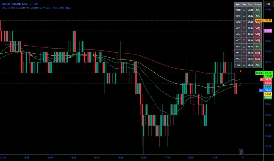
Turtle Trader StrategyTurtle Trader Strategy :
Introduction :
This strategy is based on the well known « Turtle Trader Strategy », that has proven itself over the years. It sends long and short signals with pyramid orders of up to 5, meaning that the strategy can trigger up to 5 orders in the same direction. Good risk and money management.
It's important to note that the strategy combines 2 systems working together (S1 and S2). Let’s describe the specific features of this strategy.
1/ Position size :
Position size is very important for turtle traders to manage risk properly. This position sizing strategy adapts to market volatility and to account (gains and losses). It’s based on ATR (Average True Range) which can also be called « N ». Its length is per default 20.
ATR(20) = (previous_atr(20)*19 + actual_true_range)/20
The number of units to buy is :
Unit = 1% * account/(ATR(20)*dollar_per_point)
where account is the actual account value and dollar_per_point is the variation in dollar of the asset with a 1 point move.
Depending on your risk aversion, you can increase the percentage of your account, but turtle traders default to 1%. If you trade contracts, units must be rounded down by default.
There is also an additional rule to reduce the risk if the value of the account falls below the initial capital : in this case and only in this case, account in the unit formula must be replace by :
account = actual_account*actual_account/initial capital
2/ Open a position :
2 systems are working together :
System 1 : Entering a new 20 day breakout
System 2 : Entering a new 55 day breakout
A breakout is a new high or new low. If it’s a new high, we open long position and vice versa if it’s a new low we enter in short position.
We add an additional rule :
System 1 : Breakout is ignored if last long/short position was a winner
System 2 : All signals are taken
This additional rule allows the trader to be in the major trends if the system 1 signal has been skipped. If a signal for system 1 has been skipped, and next candle is also a new 20 day breakout, S1 doesn’t give a signal. We have to wait S2 signal or wait for a candle that doesn’t make a new breakout to reactivate S1.
3/ Pyramid orders :
Turtle Strategy allows us to add extra units to the position if the price moves in our favor. I've configured the strategy to allow up to 5 orders to be added in the same direction. So if the price varies from 0.5*ATR(20) , we add units with the position size formula. Note that the value of account will be replaced by "remaining_account", i.e. the cash remaining in our account after subtracting the value of open positions.
4/ Stop Loss :
We set a stop loss at 1.5*ATR(20) below the entry price for longs and above the entry price for shorts. If pyramid units are added, the stop is increased/decreased by 0.5*ATR(20). Note that if SL is configured for a loss of more than 10%, we set the SL to 10% for the first entry order to avoid big losses. This configuration does not work for pyramid orders as SL moves by 0.5*ATR(20).
5/ Exit signals :
System 1 :
Exit long on a 10 day low
Exit short on a 10 day high
System 2 :
Exit long on a 20 day low
Exit short on a 20 day high
6/ What types of orders are placed ?
To enter in a position, stop orders are placed meaning that we place orders that will be automatically triggered by the signal at the exact breakout price. Stop loss and exit signals are also stop orders. Pyramid orders are market orders which will be triggered at the opening of the next candle to avoid repainting.
PARAMETERS :
Risk % of capital : Percentage used in the position size formula. Default is 1%
ATR period : ATR length used to calculate ATR. Default is 20
Stop ATR : Parameters used to fix stop loss. Default is 1.5 meaning that stop loss will be set at : buy_price - 1.5*ATR(20) for long and buy_price + 1.5*ATR(20) for short. Turtle traders default is 2 but 1.5 is better for cryptocurrency as there is a huge volatility.
S1 Long : System 1 breakout length for long. Default is 20
S2 Long : System 2 breakout length for long. Default is 55
S1 Long Exit : System 1 breakout length to exit long. Default is 10
S2 Long Exit : System 2 breakout length to exit long. Default is 20
S1 Short : System 1 breakout length for short. Default is 15
S2 Short : System 2 breakout length for short. Default is 55
S1 Short Exit : System 1 breakout length to exit short. Default is 7
S2 Short Exit : System 2 breakout length to exit short. Default is 20
Initial capital : $1000
Fees : Interactive Broker fees apply to this strategy. They are set at 0.18% of the trade value.
Slippage : 3 ticks or $0.03 per trade. Corresponds to the latency time between the moment the signal is received and the moment the order is executed by the broker.
Pyramiding : Number of orders that can be passed in the same direction. Default is 5.
Important : Turtle traders don't trade crypto. For this specific asset type, I modify some parameters such as SL and Short S1 in order to maximize return while limiting drawdown. This strategy is the most optimal on BINANCE:BTCUSD in 1D timeframe with the parameters set per default. If you want to use this strategy for a different crypto please adapt parameters.
NOTE :
It's important to note that the first entry order (long or short) will be the largest. Subsequent pyramid orders will have fewer units than the first order. We've set a maximum SL for the first order of 10%, meaning that you won't lose more than 10% of the value of your first order. However, it is possible to lose more on your pyramid orders, as the SL is increased/decreased by 0.5*ATR(20), which does not secure a loss of more than 10% on your pyramid orders. The risk remains well managed because the value of these orders is less than the value of the first order. Remain vigilant to this small detail and adjust your risk according to your risk aversion.
Enjoy the strategy and don’t forget to take the trade :)
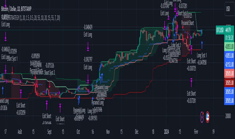
Rollover LTEThis indicator shows where price needs to be and when in order to cause the 20-sma and 50-sma moving averages to change directions. A change in direction requires the slope of a moving average to change from negative to positive or from positive to negative. When a moving average changes direction, it can be said that it has “rolled over” or “rolled up,” with the latter only applying if slope went from negative to positive.
Theory:
In order to solve for the price of the current bar that will cause the moving average to roll up, the slope from the previous bar’s average to the current bar’s average must be set equal to zero which is to say that the averages must be the same.
For the 20-sma, the equation simply stated in words is as follows:
Current MA as a function of current price and previous 19 values = previous MA which is fixed based on previous 20 values
The denominators which are both 20 cancel and the previous 19 values cancel. What’s left is current price on the left side and the value from 20 bars ago on the right.
Current price = value from 20 bars ago
and since the equation was set up for solving for the price of the current bar that will cause the MA to roll over
Rollover price = value from 20 bars ago
This makes plotting rollover price, both current and forecasted, fairly simple, as it’s merely the closing price plotted with an offset to the right the same distance as the moving average length.
Application:
The 20-sma and 50-sma rollover prices are plotted because they are considered to be the two most important moving averages for rollover analysis. Moving average lengths can be modified in the indicator settings. The 20-sma and 20-sma rollover price are both plotted in white and the 50-sma and 50-sma rollover price are both plotted in blue. There are two rollover prices because the 20-sma rollover price is the price that will cause the 20-sma to roll over and the 50-sma rollover price is the price that will cause the 50-sma to roll over. The one that's vertically furthest away from the current price is the one that will cause both to rollover, as should become clearer upon reading the explanation below.
The distance between the current price and the 20-sma rollover price is referred to as the “rollover strength” of the price relative to the 20-sma. A large disparity between the current price and the rollover price suggests bearishness (negative rollover strength) if the rollover price is overhead because price would need to travel all that distance in order to cause the moving average to roll up. If the rollover price and price are converging, as is often the case, a change in moving average and price direction becomes more plausible. The rollover strengths of the 20-sma and 50-sma are added together to calculate the Rollover Strength and if a negative number is the result then the background color of the plot cloud turns red. If the result is positive, it turns green. Rollover Strength is plotted below price as a separate indicator in this publication for reference only and it's not part of this indicator. It does not look much different from momentum indicators. The code is below if anybody wants to try to use it. The important thing is that the distances between the rollover prices and the price action are kept in mind as having shrinking, growing, or neutral bearish and bullish effects on current and forecasted price direction. Trades should not be entered based on cloud colorization changes alone.
If you are about to crash into a wall of the 20-sma rollover price, as is indicated on the chart by the green arrow, you might consider going long so long as the rollover strength, both current and forecasted, of the 50-sma isn’t questionably bearish. This is subject to analysis and interpretation. There was a 20-sma rollover wall as indicated with yellow arrow, but the bearish rollover strength of the 50-sma was growing and forecasted to remain strong for a while at that time so a long entry would have not been suggested by both rollover prices. If you are about to crash into both the 20-sma and 50-sma rollover prices at the same time (not shown on this chart), that’s a good time to place a trade in anticipation of both slopes changing direction. You may, in the case of this chart, see that a 20-sma rollover wall precedes a 50-sma rollover convergence with price and anticipate a cascade which turned out to be the case with this recent NQ rally.
Price exiting the cloud entirely to either the upside or downside has strong implications. When exiting to the downside, the 20-sma and 50-sma have both rolled over and price is below both of them. The same is true for upside exits. Re-entering the cloud after a rally may indicate a reversal is near, especially if the forecasted rollover prices, particularly the 50-sma, agree.
This indicator should be used in conjunction with other technical analysis tools.
Additional Notes:
The original version of this script which will not be published was much heavier, cluttered, and is not as useful. This is the light version, hence the “LTE” suffix.
LTE stands for “long-term evolution” in telecommunications, not “light.”
Bar colorization (red, yellow, and green bars) was added using the MACD Hybrid BSH script which is another script I’ve published.
If you’re not sure what a bar is, it’s the same thing as a candle or a data point on a line chart. Every vertical line showing price action on the chart above is a bar and it is a bar chart.
sma = simple moving average
Rollover Strength Script:
// This source code is subject to the terms of the Mozilla Public License 2.0 at mozilla.org
// © Skipper86
//@version=5
indicator(title="Rollover Strength", shorttitle="Rollover Strength", overlay=false)
source = input.source(close)
length1 = input.int(20, "Length 1", minval=1)
length2 = input.int(50, "Length 2", minval=1)
RolloverPrice1 = source
RolloverPrice2 = source
RolloverStrength1 = source-RolloverPrice1
RolloverStrength2 = source-RolloverPrice2
RolloverStrength = RolloverStrength1 + RolloverStrength2
Color1 = color.rgb(155, 155, 155, 0)
Color2 = color.rgb(0, 0, 200, 0)
Color3 = color.rgb(0, 200, 0, 0)
plot(RolloverStrength, title="Rollover Strength", color=Color3)
hline(0, "Middle Band", color=Color1)
//End of Rollover Strength Script

Bifurcation Zone - CAEBifurcation Zone — Cognitive Adversarial Engine (BZ-CAE)
Bifurcation Zone — CAE (BZ-CAE) is a next-generation divergence detection system enhanced by a Cognitive Adversarial Engine that evaluates both sides of every potential trade before presenting signals. Unlike traditional divergence indicators that show every price-oscillator disagreement regardless of context, BZ-CAE applies comprehensive market-state intelligence to identify only the divergences that occur in favorable conditions with genuine probability edges.
The system identifies structural bifurcation points — critical junctures where price and momentum disagree, signaling potential reversals or continuations — then validates these opportunities through five interconnected intelligence layers: Trend Conviction Scoring , Directional Momentum Alignment , Multi-Factor Exhaustion Modeling , Adversarial Validation , and Confidence Scoring . The result is a selective, context-aware signal system that filters noise and highlights high-probability setups.
This is not a "buy the arrow" indicator. It's a decision support framework that teaches you how to read market state, evaluate divergence quality, and make informed trading decisions based on quantified intelligence rather than hope.
What Sets BZ-CAE Apart: Technical Architecture
The Problem With Traditional Divergence Indicators
Most divergence indicators operate on a simple rule: if price makes a higher high and RSI makes a lower high, show a bearish signal. If price makes a lower low and RSI makes a higher low, show a bullish signal. This creates several critical problems:
Context Blindness : They show counter-trend signals in powerful trends that rarely reverse, leading to repeated losses as you fade momentum.
Signal Spam : Every minor price-oscillator disagreement generates an alert, overwhelming you with low-quality setups and creating analysis paralysis.
No Quality Ranking : All signals are treated identically. A marginal divergence in choppy conditions receives the same visual treatment as a high-conviction setup at a major exhaustion point.
Single-Sided Evaluation : They ask "Is this a good long?" without checking if the short case is overwhelmingly stronger, leading you into obvious bad trades.
Static Configuration : You manually choose RSI 14 or Stochastic 14 and hope it works, with no systematic way to validate if that's optimal for your instrument.
BZ-CAE's Solution: Cognitive Adversarial Intelligence
BZ-CAE solves these problems through an integrated five-layer intelligence architecture:
1. Trend Conviction Score (TCS) — 0 to 1 Scale
Most indicators check if ADX is above 25 to determine "trending" conditions. This binary approach misses nuance. TCS is a weighted composite metric:
Formula : 0.35 × normalize(ADX, 10, 35) + 0.35 × structural_strength + 0.30 × htf_alignment
Structural Strength : 10-bar SMA of consecutive directional bars. Captures persistence — are bulls or bears consistently winning?
HTF Alignment : Multi-timeframe EMA stacking (20/50/100/200). When all EMAs align in the same direction, you're in institutional trend territory.
Purpose : Quantifies how "locked in" the trend is. When TCS exceeds your threshold (default 0.80), the system knows to avoid counter-trend trades unless other factors override.
Interpretation :
TCS > 0.85: Very strong trend — counter-trading is extremely high risk
TCS 0.70-0.85: Strong trend — favor continuation, require exhaustion for reversals
TCS 0.50-0.70: Moderate trend — context matters, both directions viable
TCS < 0.50: Weak/choppy — reversals more viable, range-bound conditions
2. Directional Momentum Alignment (DMA) — ATR-Normalized
Formula : (EMA21 - EMA55) / ATR14
This isn't just "price above EMA" — it's a regime-aware momentum gauge. The same $100 price movement reads completely differently in high-volatility crypto versus low-volatility forex. By normalizing with ATR, DMA adapts its interpretation to current market conditions.
Purpose : Quantifies the directional "force" behind current price action. Positive = bullish push, negative = bearish push. Magnitude = strength.
Interpretation :
DMA > 0.7: Strong bullish momentum — bearish divergences risky
DMA 0.3 to 0.7: Moderate bullish bias
DMA -0.3 to 0.3: Balanced/choppy conditions
DMA -0.7 to -0.3: Moderate bearish bias
DMA < -0.7: Strong bearish momentum — bullish divergences risky
3. Multi-Factor Exhaustion Modeling — 0 to 1 Probability
Single-metric exhaustion detection (like "RSI > 80") misses complex market states. BZ-CAE aggregates five independent exhaustion signals:
Volume Spikes : Current volume versus 50-bar average
2.5x average: 0.25 weight
2.0x average: 0.15 weight
1.5x average: 0.10 weight
Divergence Present : The fact that a divergence exists contributes 0.30 weight — structural momentum disagreement is itself an exhaustion signal.
RSI Extremes : Captures oscillator climax zones
RSI > 80 or < 20: 0.25 weight
RSI > 75 or < 25: 0.15 weight
Pin Bar Detection : Identifies rejection candles (2:1 wick-to-body ratio, indicating failed breakout attempts): 0.15 weight
Extended Runs : Consecutive bars above/below EMA20 without pullback
30+ bars: 0.15 weight (market hasn't paused to consolidate)
Total exhaustion score is the sum of all applicable weights, capped at 1.0.
Purpose : Detects when strong trends become vulnerable to reversal. High exhaustion can override trend filters, allowing counter-trend trades at genuine turning points that basic indicators would miss.
Interpretation :
Exhaustion > 0.75: High probability of climax — yellow background shading alerts you visually
Exhaustion 0.50-0.75: Moderate overextension — watch for confirmation
Exhaustion < 0.50: Fresh move — trend can continue, counter-trend trades higher risk
4. Adversarial Validation — Game Theory Applied to Trading
This is BZ-CAE's signature innovation. Before approving any signal, the engine quantifies BOTH sides of the trade simultaneously:
For Bullish Divergences , it calculates:
Bull Case Score (0-1+) :
Distance below EMA20 (pullback quality): up to 0.25
Bullish EMA alignment (close > EMA20 > EMA50): 0.25
Oversold RSI (< 40): 0.25
Volume confirmation (> 1.2x average): 0.25
Bear Case Score (0-1+) :
Price below EMA50 (structural weakness): 0.30
Very oversold RSI (< 30, indicating knife-catching): 0.20
Differential = Bull Case - Bear Case
If differential < -0.10 (default threshold), the bear case is dominating — signal is BLOCKED or ANNOTATED.
For Bearish Divergences , the logic inverts (Bear Case vs Bull Case).
Purpose : Prevents trades where you're fighting obvious strength in the opposite direction. This is institutional-grade risk management — don't just evaluate your trade, evaluate the counter-trade simultaneously.
Why This Matters : You might see a bullish divergence at a local low, but if price is deeply below major support EMAs with strong bearish momentum, you're catching a falling knife. The adversarial check catches this and blocks the signal.
5. Confidence Scoring — 0 to 1 Quality Assessment
Every signal that passes initial filters receives a comprehensive quality score:
Formula :
0.30 × normalize(TCS) // Trend context
+ 0.25 × normalize(|DMA|) // Momentum magnitude
+ 0.20 × pullback_quality // Entry distance from EMA20
+ 0.15 × state_quality // ADX + alignment + structure
+ 0.10 × divergence_strength // Slope separation magnitude
+ adversarial_bonus (0-0.30) // Your side's advantage
Purpose : Ranks setup quality for filtering and position sizing decisions. You can set a minimum confidence threshold (default 0.35) to ensure only quality setups reach your chart.
Interpretation :
Confidence > 0.70: Premium setup — consider increased position size
Confidence 0.50-0.70: Good quality — standard size
Confidence 0.35-0.50: Acceptable — reduced size or skip if conservative
Confidence < 0.35: Marginal — blocked in Filtering mode, annotated in Advisory mode
CAE Operating Modes: Learning vs Enforcement
Off : Disables all CAE logic. Raw divergence pipeline only. Use for baseline comparison.
Advisory : Shows ALL signals regardless of CAE evaluation, but annotates signals that WOULD be blocked with specific warnings (e.g., "Bull: strong downtrend (TCS=0.87)" or "Adversarial bearish"). This is your learning mode — see CAE's decision logic in action without missing educational opportunities.
Filtering : Actively blocks low-quality signals. Only setups that pass all enabled gates (Trend Filter, Adversarial Validation, Confidence Gating) reach your chart. This is your live trading mode — trust the system to enforce discipline.
CAE Filter Gates: Three-Layer Protection
When CAE is enabled, signals must pass through three independent gates (each can be toggled on/off):
Gate 1: Strong Trend Filter
If TCS ≥ tcs_threshold (default 0.80)
And signal is counter-trend (bullish in downtrend or bearish in uptrend)
And exhaustion < exhaustion_required (default 0.50)
Then: BLOCK signal
Logic: Don't fade strong trends unless the move is clearly overextended
Gate 2: Adversarial Validation
Calculate both bull case and bear case scores
If opposing case dominates by more than adv_threshold (default 0.10)
Then: BLOCK signal
Logic: Avoid trades where you're fighting obvious strength in the opposite direction
Gate 3: Confidence Gating
Calculate composite confidence score (0-1)
If confidence < min_confidence (default 0.35)
Then: In Filtering mode, BLOCK signal; in Advisory mode, ANNOTATE with warning
Logic: Only take setups with minimum quality threshold
All three gates work together. A signal must pass ALL enabled gates to fire.
Visual Intelligence System
Bifurcation Zones (Supply/Demand Blocks)
When a divergence signal fires, BZ-CAE draws a semi-transparent box extending 15 bars forward from the signal pivot:
Demand Zones (Bullish) : Theme-colored box (cyan in Cyberpunk, blue in Professional, etc.) labeled "Demand" — marks where smart money likely placed buy orders as price diverged at the low.
Supply Zones (Bearish) : Theme-colored box (magenta in Cyberpunk, orange in Professional) labeled "Supply" — marks where smart money likely placed sell orders as price diverged at the high.
Theory : Divergences represent institutional disagreement with the crowd. The crowd pushed price to an extreme (new high or low), but momentum (oscillator) is waning, indicating smart money is taking the opposite side. These zones mark order placement areas that become future support/resistance.
Use Cases :
Exit targets: Take profit when price returns to opposite-side zone
Re-entry levels: If price returns to your entry zone, consider adding
Stop placement: Place stops just beyond your zone (below demand, above supply)
Auto-Cleanup : System keeps the last 20 zones to prevent chart clutter.
Adversarial Bar Coloring — Real-Time Market Debate Heatmap
Each bar is colored based on the Bull Case vs Bear Case differential:
Strong Bull Advantage (diff > 0.3): Full theme bull color (e.g., cyan)
Moderate Bull Advantage (diff > 0.1): 50% transparency bull
Neutral (diff -0.1 to 0.1): Gray/neutral theme
Moderate Bear Advantage (diff < -0.1): 50% transparency bear
Strong Bear Advantage (diff < -0.3): Full theme bear color (e.g., magenta)
This creates a real-time visual heatmap showing which side is "winning" the market debate. When bars flip from cyan to magenta (or vice versa), you're witnessing a shift in adversarial advantage — a leading indicator of potential momentum changes.
Exhaustion Shading
When exhaustion score exceeds 0.75, the chart background displays a semi-transparent yellow highlight. This immediate visual warning alerts you that the current move is at high risk of reversal, even if trend indicators remain strong.
Visual Themes — Six Aesthetic Options
Cyberpunk : Cyan/Magenta/Yellow — High contrast, neon aesthetic, excellent for dark-themed trading environments
Professional : Blue/Orange/Green — Corporate color palette, suitable for presentations and professional documentation
Ocean : Teal/Red/Cyan — Aquatic palette, calming for extended monitoring sessions
Fire : Orange/Red/Coral — Warm aggressive colors, high energy
Matrix : Green/Red/Lime — Code aesthetic, homage to classic hacker visuals
Monochrome : White/Gray — Minimal distraction, maximum focus on price action
All visual elements (signal markers, zones, bar colors, dashboard) adapt to your selected theme.
Divergence Engine — Core Detection System
What Are Divergences?
Divergences occur when price action and momentum indicators disagree, creating structural tension that often resolves in a change of direction:
Regular Divergence (Reversal Signal) :
Bearish Regular : Price makes higher high, oscillator makes lower high → Potential trend reversal down
Bullish Regular : Price makes lower low, oscillator makes higher low → Potential trend reversal up
Hidden Divergence (Continuation Signal) :
Bearish Hidden : Price makes lower high, oscillator makes higher high → Downtrend continuation
Bullish Hidden : Price makes higher low, oscillator makes lower low → Uptrend continuation
Both types can be enabled/disabled independently in settings.
Pivot Detection Methods
BZ-CAE uses symmetric pivot detection with separate lookback and lookforward periods (default 5/5):
Pivot High : Bar where high > all highs within lookback range AND high > all highs within lookforward range
Pivot Low : Bar where low < all lows within lookback range AND low < all lows within lookforward range
This ensures structural validity — the pivot must be a clear local extreme, not just a minor wiggle.
Divergence Validation Requirements
For a divergence to be confirmed, it must satisfy:
Slope Disagreement : Price slope and oscillator slope must move in opposite directions (for regular divs) or same direction with inverted highs/lows (for hidden divs)
Minimum Slope Change : |osc_slope| > min_slope_change / 100 (default 1.0) — filters weak, marginal divergences
Maximum Lookback Range : Pivots must be within max_lookback bars (default 60) — prevents ancient, irrelevant divergences
ATR-Normalized Strength : Divergence strength = min(|price_slope| × |osc_slope| × 10, 1.0) — quantifies the magnitude of disagreement in volatility context
Regular divergences receive 1.0× weight; hidden divergences receive 0.8× weight (slightly less reliable historically).
Oscillator Options — Five Professional Indicators
RSI (Relative Strength Index) : Classic overbought/oversold momentum indicator. Best for: General purpose divergence detection across all instruments.
Stochastic : Range-bound %K momentum comparing close to high-low range. Best for: Mean reversion strategies and range-bound markets.
CCI (Commodity Channel Index) : Measures deviation from statistical mean, auto-normalized to 0-100 scale. Best for: Cyclical instruments and commodities.
MFI (Money Flow Index) : Volume-weighted RSI incorporating money flow. Best for: Volume-driven markets like stocks and crypto.
Williams %R : Inverse stochastic looking back over period, auto-adjusted to 0-100. Best for: Reversal detection at extremes.
Each oscillator has adjustable length (2-200, default 14) and smoothing (1-20, default 1). You also set overbought (50-100, default 70) and oversold (0-50, default 30) thresholds.
Signal Timing Modes — Understanding Repainting
BZ-CAE offers two timing policies with complete transparency about repainting behavior:
Realtime (1-bar, peak-anchored)
How It Works :
Detects peaks 1 bar ago using pattern: high > high AND high > high
Signal prints on the NEXT bar after peak detection (bar_index)
Visual marker anchors to the actual PEAK bar (bar_index - 1, offset -1)
Signal locks in when bar CONFIRMS (closes)
Repainting Behavior :
On the FORMING bar (before close), the peak condition may change as new prices arrive
Once bar CLOSES (barstate.isconfirmed), signal is locked permanently
This is preview/early warning behavior by design
Best For :
Active monitoring and immediate alerts
Learning the system (seeing signals develop in real-time)
Responsive entry if you're watching the chart live
Confirmed (lookforward)
How It Works :
Uses Pine Script's built-in ta.pivothigh() and ta.pivotlow() functions
Requires full pivot validation period (lookback + lookforward bars)
Signal prints pivot_lookforward bars after the actual peak (default 5-bar delay)
Visual marker anchors to the actual peak bar (offset -pivot_lookforward)
No Repainting Behavior
Best For :
Backtesting and historical analysis
Conservative entries requiring full confirmation
Automated trading systems
Swing trading with larger timeframes
Tradeoff :
Delayed entry by pivot_lookforward bars (typically 5 bars)
On a 5-minute chart, this is a 25-minute delay
On a 4-hour chart, this is a 20-hour delay
Recommendation : Use Confirmed for backtesting to verify system performance honestly. Use Realtime for live monitoring only if you're actively watching the chart and understand pre-confirmation repainting behavior.
Signal Spacing System — Anti-Spam Architecture
Even after CAE filtering, raw divergences can cluster. The spacing system enforces separation:
Three Independent Filters
1. Min Bars Between ANY Signals (default 12):
Prevents rapid-fire clustering across both directions
If last signal (bull or bear) was within N bars, block new signal
Ensures breathing room between all setups
2. Min Bars Between SAME-SIDE Signals (default 24, optional enforcement):
Prevents bull-bull or bear-bear spam
Separate tracking for bullish and bearish signal timelines
Toggle enforcement on/off
3. Min ATR Distance From Last Signal (default 0, optional):
Requires price to move N × ATR from last signal location
Ensures meaningful price movement between setups
0 = disabled, 0.5-2.0 = typical range for enabled
All three filters work independently. A signal must pass ALL enabled filters to proceed.
Practical Guidance :
Scalping (1-5m) : Any 6-10, Same-side 12-20, ATR 0-0.5
Day Trading (15m-1H) : Any 12, Same-side 24, ATR 0-1.0
Swing Trading (4H-D) : Any 20-30, Same-side 40-60, ATR 1.0-2.0
Dashboard — Real-Time Control Center
The dashboard (toggleable, four corner positions, three sizes) provides comprehensive system intelligence:
Oscillator Section
Current oscillator type and value
State: OVERBOUGHT / OVERSOLD / NEUTRAL (color-coded)
Length parameter
Cognitive Engine Section
TCS (Trend Conviction Score) :
Current value with emoji state indicator
🔥 = Strong trend (>0.75)
📊 = Moderate trend (0.50-0.75)
〰️ = Weak/choppy (<0.50)
Color: Red if above threshold (trend filter active), yellow if moderate, green if weak
DMA (Directional Momentum Alignment) :
Current value with emoji direction indicator
🐂 = Bullish momentum (>0.5)
⚖️ = Balanced (-0.5 to 0.5)
🐻 = Bearish momentum (<-0.5)
Color: Green if bullish, red if bearish
Exhaustion :
Current value with emoji warning indicator
⚠️ = High exhaustion (>0.75)
🟡 = Moderate (0.50-0.75)
✓ = Low (<0.50)
Color: Red if high, yellow if moderate, green if low
Pullback :
Quality of current distance from EMA20
Values >0.6 are ideal entry zones (not too close, not too far)
Bull Case / Bear Case (if Adversarial enabled):
Current scores for both sides of the market debate
Differential with emoji indicator:
📈 = Bull advantage (>0.2)
➡️ = Balanced (-0.2 to 0.2)
📉 = Bear advantage (<-0.2)
Last Signal Metrics Section (New Feature)
When a signal fires, this section captures and displays:
Signal type (BULL or BEAR)
Bars elapsed since signal
Confidence % at time of signal
TCS value at signal time
DMA value at signal time
Purpose : Provides a historical reference for learning. You can see what the market state looked like when the last signal fired, helping you correlate outcomes with conditions.
Statistics Section
Total Signals : Lifetime count across session
Blocked Signals : Count and percentage (filter effectiveness metric)
Bull Signals : Total bullish divergences
Bear Signals : Total bearish divergences
Purpose : System health monitoring. If blocked % is very high (>60%), filters may be too strict. If very low (<10%), filters may be too loose.
Advisory Annotations
When CAE Mode = Advisory, this section displays warnings for signals that would be blocked in Filtering mode:
Examples:
"Bull spacing: wait 8 bars"
"Bear: strong uptrend (TCS=0.87)"
"Adversarial bearish"
"Low confidence 32%"
Multiple warnings can stack, separated by " | ". This teaches you CAE's decision logic transparently.
How to Use BZ-CAE — Complete Workflow
Phase 1: Initial Setup (First Session)
Apply BZ-CAE to your chart
Select your preferred Visual Theme (Cyberpunk recommended for visibility)
Set Signal Timing to "Confirmed (lookforward)" for learning
Choose your Oscillator Type (RSI recommended for general use, length 14)
Set Overbought/Oversold to 70/30 (standard)
Enable both Regular Divergence and Hidden Divergence
Set Pivot Lookback/Lookforward to 5/5 (balanced structure)
Enable CAE Intelligence
Set CAE Mode to "Advisory" (learning mode)
Enable all three CAE filters: Strong Trend Filter , Adversarial Validation , Confidence Gating
Enable Show Dashboard , position Top Right, size Normal
Enable Draw Bifurcation Zones and Adversarial Bar Coloring
Phase 2: Learning Period (Weeks 1-2)
Goal : Understand how CAE evaluates market state and filters signals.
Activities :
Watch the dashboard during signals :
Note TCS values when counter-trend signals fail — this teaches you the trend strength threshold for your instrument
Observe exhaustion patterns at actual turning points — learn when overextension truly matters
Study adversarial differential at signal times — see when opposing cases dominate
Review blocked signals (orange X-crosses):
In Advisory mode, you see everything — signals that would pass AND signals that would be blocked
Check the advisory annotations to understand why CAE would block
Track outcomes: Were the blocks correct? Did those signals fail?
Use Last Signal Metrics :
After each signal, check the dashboard capture of confidence, TCS, and DMA
Journal these values alongside trade outcomes
Identify patterns: Do confidence >0.70 signals work better? Does your instrument respect TCS >0.85?
Understand your instrument's "personality" :
Trending instruments (indices, major forex) may need TCS threshold 0.85-0.90
Choppy instruments (low-cap stocks, exotic pairs) may work best with TCS 0.70-0.75
High-volatility instruments (crypto) may need wider spacing
Low-volatility instruments may need tighter spacing
Phase 3: Calibration (Weeks 3-4)
Goal : Optimize settings for your specific instrument, timeframe, and style.
Calibration Checklist :
Min Confidence Threshold :
Review confidence distribution in your signal journal
Identify the confidence level below which signals consistently fail
Set min_confidence slightly above that level
Day trading : 0.35-0.45
Swing trading : 0.40-0.55
Scalping : 0.30-0.40
TCS Threshold :
Find the TCS level where counter-trend signals consistently get stopped out
Set tcs_threshold at or slightly below that level
Trending instruments : 0.85-0.90
Mixed instruments : 0.80-0.85
Choppy instruments : 0.75-0.80
Exhaustion Override Level :
Identify exhaustion readings that marked genuine reversals
Set exhaustion_required just below the average
Typical range : 0.45-0.55
Adversarial Threshold :
Default 0.10 works for most instruments
If you find CAE is too conservative (blocking good trades), raise to 0.15-0.20
If signals are still getting caught in opposing momentum, lower to 0.07-0.09
Spacing Parameters :
Count bars between quality signals in your journal
Set min bars ANY to ~60% of that average
Set min bars SAME-SIDE to ~120% of that average
Scalping : Any 6-10, Same 12-20
Day trading : Any 12, Same 24
Swing : Any 20-30, Same 40-60
Oscillator Selection :
Try different oscillators for 1-2 weeks each
Track win rate and average winner/loser by oscillator type
RSI : Best for general use, clear OB/OS
Stochastic : Best for range-bound, mean reversion
MFI : Best for volume-driven markets
CCI : Best for cyclical instruments
Williams %R : Best for reversal detection
Phase 4: Live Deployment
Goal : Disciplined execution with proven, calibrated system.
Settings Changes :
Switch CAE Mode from Advisory to Filtering
System now actively blocks low-quality signals
Only setups passing all gates reach your chart
Keep Signal Timing on Confirmed for conservative entries
OR switch to Realtime if you're actively monitoring and want faster entries (accept pre-confirmation repaint risk)
Use your calibrated thresholds from Phase 3
Enable high-confidence alerts: "⭐ High Confidence Bullish/Bearish" (>0.70)
Trading Discipline Rules :
Respect Blocked Signals :
If CAE blocks a trade you wanted to take, TRUST THE SYSTEM
Don't manually override — if you consistently disagree, return to Phase 2/3 calibration
The block exists because market state failed intelligence checks
Confidence-Based Position Sizing :
Confidence >0.70: Standard or increased size (e.g., 1.5-2.0% risk)
Confidence 0.50-0.70: Standard size (e.g., 1.0% risk)
Confidence 0.35-0.50: Reduced size (e.g., 0.5% risk) or skip if conservative
TCS-Based Management :
High TCS + counter-trend signal: Use tight stops, quick exits (you're fading momentum)
Low TCS + reversal signal: Use wider stops, trail aggressively (genuine reversal potential)
Exhaustion Awareness :
Exhaustion >0.75 (yellow shading): Market is overextended, reversal risk is elevated — consider early exit or tighter trailing stops even on winning trades
Exhaustion <0.30: Continuation bias — hold for larger move, wide trailing stops
Adversarial Context :
Strong differential against you (e.g., bullish signal with bear diff <-0.2): Use very tight stops, consider skipping
Strong differential with you (e.g., bullish signal with bull diff >0.2): Trail aggressively, this is your tailwind
Practical Settings by Timeframe & Style
Scalping (1-5 Minute Charts)
Objective : High frequency, tight stops, quick reversals in fast-moving markets.
Oscillator :
Type: RSI or Stochastic (fast response to quick moves)
Length: 9-11 (more responsive than standard 14)
Smoothing: 1 (no lag)
OB/OS: 65/35 (looser thresholds ensure frequent crossings in fast conditions)
Divergence :
Pivot Lookback/Lookforward: 3/3 (tight structure, catch small swings)
Max Lookback: 40-50 bars (recent structure only)
Min Slope Change: 0.8-1.0 (don't be overly strict)
CAE :
Mode: Advisory first (learn), then Filtering
Min Confidence: 0.30-0.35 (lower bar for speed, accept more signals)
TCS Threshold: 0.70-0.75 (allow more counter-trend opportunities)
Exhaustion Required: 0.45-0.50 (moderate override)
Strong Trend Filter: ON (still respect major intraday trends)
Adversarial: ON (critical for scalping protection — catches bad entries quickly)
Spacing :
Min Bars ANY: 6-10 (fast pace, many setups)
Min Bars SAME-SIDE: 12-20 (prevent clustering)
Min ATR Distance: 0 or 0.5 (loose)
Timing : Realtime (speed over precision, but understand repaint risk)
Visuals :
Signal Size: Tiny (chart clarity in busy conditions)
Show Zones: Optional (can clutter on low timeframes)
Bar Coloring: ON (helps read momentum shifts quickly)
Dashboard: Small size (corner reference, not main focus)
Key Consideration : Scalping generates noise. Even with CAE, expect lower win rate (45-55%) but aim for favorable R:R (2:1 or better). Size conservatively.
Day Trading (15-Minute to 1-Hour Charts)
Objective : Balance quality and frequency. Standard divergence trading approach.
Oscillator :
Type: RSI or MFI (proven reliability, volume confirmation with MFI)
Length: 14 (industry standard, well-studied)
Smoothing: 1-2
OB/OS: 70/30 (classic levels)
Divergence :
Pivot Lookback/Lookforward: 5/5 (balanced structure)
Max Lookback: 60 bars
Min Slope Change: 1.0 (standard strictness)
CAE :
Mode: Filtering (enforce discipline from the start after brief Advisory learning)
Min Confidence: 0.35-0.45 (quality filter without being too restrictive)
TCS Threshold: 0.80-0.85 (respect strong trends)
Exhaustion Required: 0.50 (balanced override threshold)
Strong Trend Filter: ON
Adversarial: ON
Confidence Gating: ON (all three filters active)
Spacing :
Min Bars ANY: 12 (breathing room between all setups)
Min Bars SAME-SIDE: 24 (prevent bull/bear clusters)
Min ATR Distance: 0-1.0 (optional refinement, typically 0.5-1.0)
Timing : Confirmed (1-bar delay for reliability, no repainting)
Visuals :
Signal Size: Tiny or Small
Show Zones: ON (useful reference for exits/re-entries)
Bar Coloring: ON (context awareness)
Dashboard: Normal size (full visibility)
Key Consideration : This is the "sweet spot" timeframe for BZ-CAE. Market structure is clear, CAE has sufficient data, and signal frequency is manageable. Expect 55-65% win rate with proper execution.
Swing Trading (4-Hour to Daily Charts)
Objective : Quality over quantity. High conviction only. Larger stops and targets.
Oscillator :
Type: RSI or CCI (robust on higher timeframes, smooth longer waves)
Length: 14-21 (capture larger momentum swings)
Smoothing: 1-3
OB/OS: 70/30 or 75/25 (strict extremes)
Divergence :
Pivot Lookback/Lookforward: 5/5 or 7/7 (structural purity, major swings only)
Max Lookback: 80-100 bars (broader historical context)
Min Slope Change: 1.2-1.5 (require strong, undeniable divergence)
CAE :
Mode: Filtering (strict enforcement, premium setups only)
Min Confidence: 0.40-0.55 (high bar for entry)
TCS Threshold: 0.85-0.95 (very strong trend protection — don't fade established HTF trends)
Exhaustion Required: 0.50-0.60 (higher bar for override — only extreme exhaustion justifies counter-trend)
Strong Trend Filter: ON (critical on HTF)
Adversarial: ON (avoid obvious bad trades)
Confidence Gating: ON (quality gate essential)
Spacing :
Min Bars ANY: 20-30 (substantial separation)
Min Bars SAME-SIDE: 40-60 (significant breathing room)
Min ATR Distance: 1.0-2.0 (require meaningful price movement)
Timing : Confirmed (purity over speed, zero repaint for swing accuracy)
Visuals :
Signal Size: Small or Normal (clear markers on zoomed-out view)
Show Zones: ON (important HTF levels)
Bar Coloring: ON (long-term trend awareness)
Dashboard: Normal or Large (comprehensive analysis)
Key Consideration : Swing signals are rare but powerful. Expect 2-5 signals per month per instrument. Win rate should be 60-70%+ due to stringent filtering. Position size can be larger given confidence.
Dashboard Interpretation Reference
TCS (Trend Conviction Score) States
0.00-0.50: Weak/Choppy
Emoji: 〰️
Color: Green/cyan
Meaning: No established trend. Range-bound or consolidating. Both reversal and continuation signals viable.
Action: Reversals (regular divs) are safer. Use wider profit targets (market has room to move). Consider mean reversion strategies.
0.50-0.75: Moderate Trend
Emoji: 📊
Color: Yellow/neutral
Meaning: Developing trend but not locked in. Context matters significantly.
Action: Check DMA and exhaustion. If DMA confirms trend and exhaustion is low, favor continuation (hidden divs). If exhaustion is high, reversals are viable.
0.75-0.85: Strong Trend
Emoji: 🔥
Color: Orange/warning
Meaning: Well-established trend with persistence. Counter-trend is high risk.
Action: Require exhaustion >0.50 for counter-trend entries. Favor continuation signals. Use tight stops on counter-trend attempts.
0.85-1.00: Very Strong Trend
Emoji: 🔥🔥
Color: Red/danger (if counter-trading)
Meaning: Locked-in institutional trend. Extremely high risk to fade.
Action: Avoid counter-trend unless exhaustion >0.75 (yellow shading). Focus exclusively on continuation opportunities. Momentum is king here.
DMA (Directional Momentum Alignment) Zones
-2.0 to -1.0: Strong Bearish Momentum
Emoji: 🐻🐻
Color: Dark red
Meaning: Powerful downside force. Sellers are in control.
Action: Bullish divergences are counter-momentum (high risk). Bearish divergences are with-momentum (lower risk). Size down on longs.
-0.5 to 0.5: Neutral/Balanced
Emoji: ⚖️
Color: Gray/neutral
Meaning: No strong directional bias. Choppy or consolidating.
Action: Both directions have similar probability. Focus on confidence score and adversarial differential for edge.
1.0 to 2.0: Strong Bullish Momentum
Emoji: 🐂🐂
Color: Bright green/cyan
Meaning: Powerful upside force. Buyers are in control.
Action: Bearish divergences are counter-momentum (high risk). Bullish divergences are with-momentum (lower risk). Size down on shorts.
Exhaustion States
0.00-0.50: Fresh Move
Emoji: ✓
Color: Green
Meaning: Trend is healthy, not overextended. Room to run.
Action: Counter-trend trades are premature. Favor continuation. Hold winners for larger moves. Avoid early exits.
0.50-0.75: Mature Move
Emoji: 🟡
Color: Yellow
Meaning: Move is aging. Watch for signs of climax.
Action: Tighten trailing stops on winning trades. Be ready for reversals. Don't add to positions aggressively.
0.75-0.85: High Exhaustion
Emoji: ⚠️
Color: Orange
Background: Yellow shading appears
Meaning: Move is overextended. Reversal risk elevated significantly.
Action: Counter-trend reversals are higher probability. Consider early exits on with-trend positions. Size up on reversal divergences (if CAE allows).
0.85-1.00: Critical Exhaustion
Emoji: ⚠️⚠️
Color: Red
Background: Yellow shading intensifies
Meaning: Climax conditions. Reversal imminent or underway.
Action: Aggressive reversal trades justified. Exit all with-trend positions. This is where major turns occur.
Confidence Score Tiers
0.00-0.30: Low Quality
Color: Red
Status: Blocked in Filtering mode
Action: Skip entirely. Setup lacks fundamental quality across multiple factors.
0.30-0.50: Moderate Quality
Color: Yellow/orange
Status: Marginal — passes in Filtering only if >min_confidence
Action: Reduced position size (0.5-0.75% risk). Tight stops. Conservative profit targets. Skip if you're selective.
0.50-0.70: High Quality
Color: Green/cyan
Status: Good setup across most quality factors
Action: Standard position size (1.0-1.5% risk). Normal stops and targets. This is your bread-and-butter trade.
0.70-1.00: Premium Quality
Color: Bright green/gold
Status: Exceptional setup — all factors aligned
Visual: Double confidence ring appears
Action: Consider increased position size (1.5-2.0% risk, maximum). Wider stops. Larger targets. High probability of success. These are rare — capitalize when they appear.
Adversarial Differential Interpretation
Bull Differential > 0.3 :
Visual: Strong cyan/green bar colors
Meaning: Bull case strongly dominates. Buyers have clear advantage.
Action: Bullish divergences favored (with-advantage). Bearish divergences face headwind (reduce size or skip). Momentum is bullish.
Bull Differential 0.1 to 0.3 :
Visual: Moderate cyan/green transparency
Meaning: Moderate bull advantage. Buyers have edge but not overwhelming.
Action: Both directions viable. Slight bias toward longs.
Differential -0.1 to 0.1 :
Visual: Gray/neutral bars
Meaning: Balanced debate. No clear advantage either side.
Action: Rely on other factors (confidence, TCS, exhaustion) for direction. Adversarial is neutral.
Bear Differential -0.3 to -0.1 :
Visual: Moderate red/magenta transparency
Meaning: Moderate bear advantage. Sellers have edge but not overwhelming.
Action: Both directions viable. Slight bias toward shorts.
Bear Differential < -0.3 :
Visual: Strong red/magenta bar colors
Meaning: Bear case strongly dominates. Sellers have clear advantage.
Action: Bearish divergences favored (with-advantage). Bullish divergences face headwind (reduce size or skip). Momentum is bearish.
Last Signal Metrics — Post-Trade Analysis
After a signal fires, dashboard captures:
Type : BULL or BEAR
Bars Ago : How long since signal (updates every bar)
Confidence : What was the quality score at signal time
TCS : What was trend conviction at signal time
DMA : What was momentum alignment at signal time
Use Case : Post-trade journaling and learning.
Example: "BULL signal 12 bars ago. Confidence: 68%, TCS: 0.42, DMA: -0.85"
Analysis : This was a bullish reversal (regular div) with good confidence, weak trend (TCS), but strong bearish momentum (DMA). The bet was that momentum would reverse — a counter-momentum play requiring exhaustion confirmation. Check if exhaustion was high at that time to justify the entry.
Track patterns:
Do your best trades have confidence >0.65?
Do low-TCS signals (<0.50) work better for you?
Are you more successful with-momentum (DMA aligned with signal) or counter-momentum?
Troubleshooting Guide
Problem: No Signals Appearing
Symptoms : Chart loads, dashboard shows metrics, but no divergence signals fire.
Diagnosis Checklist :
Check dashboard oscillator value : Is it crossing OB/OS levels (70/30)? If oscillator stays in 40-60 range constantly, it can't reach extremes needed for divergence detection.
Are pivots forming? : Look for local swing highs/lows on your chart. If price is in tight consolidation, pivots may not meet lookback/lookforward requirements.
Is spacing too tight? : Check "Last Signal" metrics — how many bars since last signal? If <12 and your min_bars_ANY is 12, spacing filter is blocking.
Is CAE blocking everything? : Check dashboard Statistics section — what's the blocked signal count? High blocks indicate overly strict filters.
Solutions :
Loosen OB/OS Temporarily :
Try 65/35 to verify divergence detection works
If signals appear, the issue was threshold strictness
Gradually tighten back to 67/33, then 70/30 as appropriate
Lower Min Confidence :
Try 0.25-0.30 (diagnostic level)
If signals appear, filter was too strict
Raise gradually to find sweet spot (0.35-0.45 typical)
Disable Strong Trend Filter Temporarily :
Turn off in CAE settings
If signals appear, TCS threshold was blocking everything
Re-enable and lower TCS_threshold to 0.70-0.75
Reduce Min Slope Change :
Try 0.7-0.8 (from default 1.0)
Allows weaker divergences through
Helpful on low-volatility instruments
Widen Spacing :
Set min_bars_ANY to 6-8
Set min_bars_SAME_SIDE to 12-16
Reduces time between allowed signals
Check Timing Mode :
If using Confirmed, remember there's a pivot_lookforward delay (5+ bars)
Switch to Realtime temporarily to verify system is working
Realtime has no delay but repaints
Verify Oscillator Settings :
Length 14 is standard but might not fit all instruments
Try length 9-11 for faster response
Try length 18-21 for slower, smoother response
Problem: Too Many Signals (Signal Spam)
Symptoms : Dashboard shows 50+ signals in Statistics, confidence scores mostly <0.40, signals clustering close together.
Solutions :
Raise Min Confidence :
Try 0.40-0.50 (quality filter)
Blocks bottom-tier setups
Targets top 50-60% of divergences only
Tighten OB/OS :
Use 70/30 or 75/25
Requires more extreme oscillator readings
Reduces false divergences in mid-range
Increase Min Slope Change :
Try 1.2-1.5 (from default 1.0)
Requires stronger, more obvious divergences
Filters marginal slope disagreements
Raise TCS Threshold :
Try 0.85-0.90 (from default 0.80)
Stricter trend filter blocks more counter-trend attempts
Favors only strongest trend alignment
Enable ALL CAE Gates :
Turn on Trend Filter + Adversarial + Confidence
Triple-layer protection
Blocks aggressively — expect 20-40% reduction in signals
Widen Spacing :
min_bars_ANY: 15-20 (from 12)
min_bars_SAME_SIDE: 30-40 (from 24)
Creates substantial breathing room
Switch to Confirmed Timing :
Removes realtime preview noise
Ensures full pivot validation
5-bar delay filters many false starts
Problem: Signals in Strong Trends Get Stopped Out
Symptoms : You take a bullish divergence in a downtrend (or bearish in uptrend), and it immediately fails. Dashboard showed high TCS at the time.
Analysis : This is INTENDED behavior — CAE is protecting you from low-probability counter-trend trades.
Understanding :
Check Last Signal Metrics in dashboard — what was TCS when signal fired?
If TCS was >0.85 and signal was counter-trend, CAE correctly identified it as high risk
Strong trends rarely reverse cleanly without major exhaustion
Your losses here are the system working as designed (blocking bad odds)
If You Want to Override (Not Recommended) :
Lower TCS_threshold to 0.70-0.75 (allows more counter-trend)
Lower exhaustion_required to 0.40 (easier override)
Disable Strong Trend Filter entirely (very risky)
Better Approach :
TRUST THE FILTER — it's preventing costly mistakes
Wait for exhaustion >0.75 (yellow shading) before counter-trending strong TCS
Focus on continuation signals (hidden divs) in high-TCS environments
Use Advisory mode to see what CAE is blocking and learn from outcomes
Problem: Adversarial Blocking Seems Wrong
Symptoms : You see a divergence that "looks good" visually, but CAE blocks with "Adversarial bearish/bullish" warning.
Diagnosis :
Check dashboard Bull Case and Bear Case scores at that moment
Look at Differential value
Check adversarial bar colors — was there strong coloring against your intended direction?
Understanding :
Adversarial catches "obvious" opposing momentum that's easy to miss
Example: Bullish divergence at a local low, BUT price is deeply below EMA50, bearish momentum is strong, and RSI shows knife-catching conditions
Bull Case might be 0.20 while Bear Case is 0.55
Differential = -0.35, far beyond threshold
Block is CORRECT — you'd be fighting overwhelming opposing flow
If You Disagree Consistently
Review blocked signals on chart — scroll back and check outcomes
Did those blocked signals actually work, or did they fail as adversarial predicted?
Raise adv_threshold to 0.15-0.20 (more permissive, allows closer battles)
Disable Adversarial Validation temporarily (diagnostic) to isolate its effect
Use Advisory mode to learn adversarial patterns over 50-100 signals
Remember : Adversarial is conservative BY DESIGN. It prevents "obvious" bad trades where you're fighting strong strength the other way.
Problem: Dashboard Not Showing or Incomplete
Solutions :
Toggle "Show Dashboard" to ON in settings
Try different dashboard sizes (Small/Normal/Large)
Try different positions (Top Left/Right, Bottom Left/Right) — might be off-screen
Some sections require CAE Enable = ON (Cognitive Engine section won't appear if CAE is disabled)
Statistics section requires at least 1 lifetime signal to populate
Check that visual theme is set (dashboard colors adapt to theme)
Problem: Performance Lag, Chart Freezing
Symptoms : Chart loading is slow, indicator calculations cause delays, pinch-to-zoom lags.
Diagnosis : Visual features are computationally expensive, especially adversarial bar coloring (recalculates every bar).
Solutions (In Order of Impact) :
Disable Adversarial Bar Coloring (MOST EXPENSIVE):
Turn OFF "Adversarial Bar Coloring" in settings
This is the single biggest performance drain
Immediate improvement
Reduce Vertical Lines :
Lower "Keep last N vertical lines" to 20-30
Or set to 0 to disable entirely
Moderate improvement
Disable Bifurcation Zones :
Turn OFF "Draw Bifurcation Zones"
Reduces box drawing calculations
Moderate improvement
Set Dashboard Size to Small :
Smaller dashboard = fewer cells = less rendering
Minor improvement
Use Shorter Max Lookback :
Reduce max_lookback to 40-50 (from 60+)
Fewer bars to scan for divergences
Minor improvement
Disable Exhaustion Shading :
Turn OFF "Show Market State"
Removes background coloring calculations
Minor improvement
Extreme Performance Mode :
Disable ALL visual enhancements
Keep only triangle markers
Dashboard Small or OFF
Use Minimal theme if available
Problem: Realtime Signals Repainting
Symptoms : You see a signal appear, but on next bar it disappears or moves.
Explanation :
Realtime mode detects peaks 1 bar ago: high > high AND high > high
On the FORMING bar (before close), this condition can change as new prices arrive
Example: At 10:05, high (10:04 bar) was 100, current high is 99 → peak detected
At 10:05:30, new high of 101 arrives → peak condition breaks → signal disappears
At 10:06 (bar close), final high is 101 → no peak at 10:04 anymore → signal gone permanently
This is expected behavior for realtime responsiveness. You get preview/early warning, but it's not locked until bar confirms.
Solutions :
Use Confirmed Timing :
Switch to "Confirmed (lookforward)" mode
ZERO repainting — pivot must be fully validated
5-bar delay (pivot_lookforward)
What you see in history is exactly what would have appeared live
Accept Realtime Repaint as Tradeoff :
Keep Realtime mode for speed and alerts
Understand that pre-confirmation signals may vanish
Only trade signals that CONFIRM at bar close (check barstate.isconfirmed)
Use for live monitoring, NOT for backtesting
Trade Only After Confirmation :
In Realtime mode, wait 1 full bar after signal appears before entering
If signal survives that bar close, it's locked
This adds 1-bar delay but removes repaint risk
Recommendation : Use Confirmed for backtesting and conservative trading. Use Realtime only for active monitoring with full understanding of preview behavior.
Risk Management Integration
BZ-CAE is a signal generation system, not a complete trading strategy. You must integrate proper risk management:
Position Sizing by Confidence
Confidence 0.70-1.00 (Premium) :
Risk: 1.5-2.0% of account (MAXIMUM)
Reasoning: High-quality setup across all factors
Still cap at 2% — even premium setups can fail
Confidence 0.50-0.70 (High Quality) :
Risk: 1.0-1.5% of account
Reasoning: Standard good setup
Your bread-and-butter risk level
Confidence 0.35-0.50 (Moderate Quality) :
Risk: 0.5-1.0% of account
Reasoning: Marginal setup, passes minimum threshold
Reduce size or skip if you're selective
Confidence <0.35 (Low Quality) :
Risk: 0% (blocked in Filtering mode)
Reasoning: Insufficient quality factors
System protects you by not showing these
Stop Placement Strategies
For Reversal Signals (Regular Divergences) :
Place stop beyond the divergence pivot plus buffer
Bullish : Stop below the divergence low - 1.0-1.5 × ATR
Bearish : Stop above the divergence high + 1.0-1.5 × ATR
Reasoning: If price breaks the pivot, divergence structure is invalidated
For Continuation Signals (Hidden Divergences) :
Place stop beyond recent swing in opposite direction
Bullish continuation : Stop below recent swing low (not the divergence pivot itself)
Bearish continuation : Stop above recent swing high
Reasoning: You're trading with trend, allow more breathing room
ATR-Based Stops :
1.5-2.0 × ATR is standard
Scale by timeframe:
Scalping (1-5m): 1.0-1.5 × ATR (tight)
Day trading (15m-1H): 1.5-2.0 × ATR (balanced)
Swing (4H-D): 2.0-3.0 × ATR (wide)
Never Use Fixed Dollar/Pip Stops :
Markets have different volatility
50-pip stop on EUR/USD ≠ 50-pip stop on GBP/JPY
Always normalize by ATR or pivot structure
Profit Targets and Scaling
Primary Target :
2-3 × ATR from entry (minimum 2:1 reward-risk)
Example : Entry at 100, ATR = 2, stop at 97 (1.5 × ATR) → target at 106 (3 × ATR) = 2:1 R:R
Scaling Out Strategy :
Take 50% off at 1.5 × ATR (secure partial profit)
Move stop to breakeven
Trail remaining 50% with 1.0 × ATR trailing stop
Let winners run if trend persists
Targets by Confidence :
High Confidence (>0.70) : Aggressive targets (3-4 × ATR), trail wider (1.5 × ATR)
Standard Confidence (0.50-0.70) : Normal targets (2-3 × ATR), standard trail (1.0 × ATR)
Low Confidence (0.35-0.50) : Conservative targets (1.5-2 × ATR), tight trail (0.75 × ATR)
Use Bifurcation Zones :
If opposite-side zone is visible on chart (from previous signal), use it as target
Example : Bullish signal at 100, prior supply zone at 110 → use 110 as target
Zones mark institutional resistance/support
Exhaustion-Based Exits :
If you're in a trade and exhaustion >0.75 develops (yellow shading), consider early exit
Market is overextended — reversal risk is high
Take profit even if target not reached
Trade Management by TCS
High TCS + Counter-Trend Trade (Risky) :
Use very tight stops (1.0-1.5 × ATR)
Conservative targets (1.5-2 × ATR)
Quick exit if trade doesn't work immediately
You're fading momentum — respect it
Low TCS + Reversal Trade (Safer) :
Use wider stops (2.0-2.5 × ATR)
Aggressive targets (3-4 × ATR)
Trail with patience
Genuine reversal potential in weak trend
High TCS + Continuation Trade (Safest) :
Standard stops (1.5-2.0 × ATR)
Very aggressive targets (4-5 × ATR)
Trail wide (1.5-2.0 × ATR)
You're with institutional momentum — let it run
Educational Value — Learning Machine Intelligence
BZ-CAE is designed as a learning platform, not just a tool:
Advisory Mode as Teacher
Most indicators are binary: signal or no signal. You don't learn WHY certain setups are better.
BZ-CAE's Advisory mode shows you EVERY potential divergence, then annotates the ones that would be blocked in Filtering mode with specific reasons:
"Bull: strong downtrend (TCS=0.87)" teaches you that TCS >0.85 makes counter-trend very risky
"Adversarial bearish" teaches you that the opposing case was dominating
"Low confidence 32%" teaches you that the setup lacked quality across multiple factors
"Bull spacing: wait 8 bars" teaches you that signals need breathing room
After 50-100 signals in Advisory mode, you internalize the CAE's decision logic. You start seeing these factors yourself BEFORE the indicator does.
Dashboard Transparency
Most "intelligent" indicators are black boxes — you don't know how they make decisions.
BZ-CAE shows you ALL metrics in real-time:
TCS tells you trend strength
DMA tells you momentum alignment
Exhaustion tells you overextension
Adversarial shows both sides of the debate
Confidence shows composite quality
You learn to interpret market state holistically, a skill applicable to ANY trading system beyond this indicator.
Divergence Quality Education
Not all divergences are equal. BZ-CAE teaches you which conditions produce high-probability setups:
Quality divergence : Regular bullish div at a low, TCS <0.50 (weak trend), exhaustion >0.75 (overextended), positive adversarial differential, confidence >0.70
Low-quality divergence : Regular bearish div at a high, TCS >0.85 (strong uptrend), exhaustion <0.30 (not overextended), negative adversarial differential, confidence <0.40
After using the system, you can evaluate divergences manually with similar intelligence.
Risk Management Discipline
Confidence-based position sizing teaches you to adjust risk based on setup quality, not emotions:
Beginners often size all trades identically
Or worse, size UP on marginal setups to "make up" for losses
BZ-CAE forces systematic sizing: premium setups get larger size, marginal setups get smaller size
This creates a probabilistic approach where your edge compounds over time.
What This Indicator Is NOT
Complete transparency about limitations and positioning:
Not a Prediction System
BZ-CAE does not predict future prices. It identifies structural divergences (price-momentum disagreements) and assesses current market state (trend, exhaustion, adversarial conditions). It tells you WHEN conditions favor a potential reversal or continuation, not WHAT WILL HAPPEN.
Markets are probabilistic. Even premium-confidence setups fail ~30-40% of the time. The system improves your probability distribution over many trades — it doesn't eliminate risk.
Not Fully Automated
This is a decision support tool, not a trading robot. You must:
Execute trades manually based on signals
Manage positions (stops, targets, trailing)
Apply discretionary judgment (news events, liquidity, context)
Integrate with your broader strategy and risk rules
The confidence scores guide position sizing, but YOU determine final risk allocation based on your account size, risk tolerance, and portfolio context.
Not Beginner-Friendly
BZ-CAE requires understanding of:
Divergence trading concepts (regular vs hidden, reversal vs continuation)
Market state interpretation (trend vs range, momentum, exhaustion)
Basic technical analysis (pivots, support/resistance, EMAs)
Risk management fundamentals (position sizing, stops, R:R)
This is designed for intermediate to advanced traders willing to invest time learning the system. If you want "buy the arrow" simplicity, this isn't the tool.
Not a Holy Grail
There is no perfect indicator. BZ-CAE filters noise and improves signal quality significantly, but:
Losing trades are inevitable (even at 70% win rate, 30% still fail)
Market conditions change rapidly (yesterday's strong trend becomes today's chop)
Black swan events occur (fundamentals override technicals)
Execution matters (slippage, fees, emotional discipline)
The system provides an EDGE, not a guarantee. Your job is to execute that edge consistently with proper risk management over hundreds of trades.
Not Financial Advice
BZ-CAE is an educational and analytical tool. All trading decisions are your responsibility. Past performance (backtested or live) does not guarantee future results. Only risk capital you can afford to lose. Consult a licensed financial advisor for investment advice specific to your situation.
Ideal Market Conditions
Best Performance Characteristics
Liquid Instruments :
Major forex pairs (EUR/USD, GBP/USD, USD/JPY)
Large-cap stocks and index ETFs (SPY, QQQ, AAPL, MSFT)
High-volume crypto (BTC, ETH)
Major commodities (Gold, Oil, Natural Gas)
Reasoning: Clean price structure, clear pivots, meaningful oscillator behavior
Trending with Consolidations :
Markets that trend for 20-40 bars, then consolidate 10-20 bars, repeat
Creates divergences at consolidation boundaries (reversals) and within trends (continuations)
Both regular and hidden divs find opportunities
5-Minute to Daily Timeframes :
Below 5m: too much noise, false pivots, CAE metrics unstable
Above daily: too few signals, edge diminishes (fundamentals dominate)
Sweet spot: 15m to 4H for most traders
Consistent Volume and Participation :
Regular trading sessions (not holidays or thin markets)
Predictable volatility patterns
Avoid instruments with sudden gaps or circuit breakers
Challenging Conditions
Extremely Low Liquidity :
Penny stocks, exotic forex pairs, low-volume crypto
Erratic pivots, unreliable oscillator readings
CAE metrics can't assess market state properly
Very Low Timeframes (1-Minute or Below) :
Dominated by market microstructure noise
Divergences are everywhere but meaningless
CAE filtering helps but still unreliable
Extended Sideways Consolidation :
100+ bars of tight range with no clear pivots
Oscillator hugs midpoint (45-55 range)
No divergences to detect
Fundamentally-Driven Gap Markets :
Earnings releases, economic data, geopolitical events
Price gaps over stops and targets
Technical structure breaks down
Recommendation: Disable trading around known events
Calculation Methodology — Technical Depth
For users who want to understand the math:
Oscillator Computation
Each oscillator type calculates differently, but all normalize to 0-100:
RSI : ta.rsi(close, length) — Standard Relative Strength Index
Stochastic : ta.stoch(high, low, close, length) — %K calculation
CCI : (ta.cci(hlc3, length) + 100) / 2 — Normalized from -100/+100 to 0-100
MFI : ta.mfi(hlc3, length) — Volume-weighted RSI equivalent
Williams %R : ta.wpr(length) + 100 — Inverted stochastic adjusted to 0-100
Smoothing: If smoothing > 1, apply ta.sma(oscillator, smoothing)
Divergence Detection Algorithm
Identify Pivots :
Price high pivot: ta.pivothigh(high, lookback, lookforward)
Price low pivot: ta.pivotlow(low, lookback, lookforward)
Oscillator high pivot: ta.pivothigh(osc, lookback, lookforward)
Oscillator low pivot: ta.pivotlow(osc, lookback, lookforward)
Store Recent Pivots :
Maintain arrays of last 10 pivots with bar indices
When new pivot confirmed, unshift to array, pop oldest if >10
Scan for Slope Disagreements :
Loop through last 5 pivots
For each pair (current pivot, historical pivot):
Check if within max_lookback bars
Calculate slopes: (current - historical) / bars_between
Regular bearish: price_slope > 0, osc_slope < 0, |osc_slope| > min_threshold
Regular bullish: price_slope < 0, osc_slope > 0, |osc_slope| > min_threshold
Hidden bearish: price_slope < 0, osc_slope > 0, osc_slope > min_threshold
Hidden bullish: price_slope > 0, osc_slope < 0, |osc_slope| > min_threshold
Important Disclaimers and Terms
Performance Disclosure
Past performance, whether backtested or live-traded, does not guarantee future results. Markets change. What works today may not work tomorrow. Hypothetical or simulated performance results have inherent limitations and do not represent actual trading.
Risk of Loss
Trading involves substantial risk of loss. Only trade with risk capital you can afford to lose entirely. The high degree of leverage often available in trading can work against you as well as for you. Leveraged trading may result in losses exceeding your initial deposit.
Not Financial Advice
BZ-CAE is an educational and analytical tool for technical analysis. It is not financial advice, investment advice, or a recommendation to buy or sell any security or instrument. All trading decisions are your sole responsibility. Consult a licensed financial advisor for advice specific to your circumstances.
Technical Indicator Limitations
BZ-CAE is a technical analysis tool based on price and volume data. It does not account for:
Fundamental analysis (earnings, economic data, financial health)
Market sentiment and positioning
Geopolitical events and news
Liquidity conditions and market microstructure changes
Regulatory changes or exchange rules
Integrate with broader analysis and strategy. Do not rely solely on technical indicators for trading decisions.
Repainting Acknowledgment
As disclosed throughout this documentation:
Realtime mode may repaint on forming bars before confirmation (by design for preview functionality)
Confirmed mode has zero repainting (fully validated pivots only)
Choose timing mode appropriate for your use case. Understand the tradeoffs.
Testing Recommendation
ALWAYS test on demo/paper accounts before committing real capital. Validate the indicator's behavior on your specific instruments and timeframes. Learn the system thoroughly in Advisory mode before using Filtering mode.
Learning Resources :
In-indicator tooltips (hover over setting names for detailed explanations)
This comprehensive publishing statement (save for reference)
User guide in script comments (top of code)
Final Word — Philosophy of BZ-CAE
BZ-CAE is not designed to replace your judgment — it's designed to enhance it.
The indicator identifies structural inflection points (bifurcations) where price and momentum disagree. The Cognitive Engine evaluates market state to determine if this disagreement is meaningful or noise. The Adversarial model debates both sides of the trade to catch obvious bad setups. The Confidence system ranks quality so you can choose your risk appetite.
But YOU still execute. YOU still manage risk. YOU still learn from outcomes.
This is intelligence amplification, not intelligence replacement.
Use Advisory mode to learn how expert traders evaluate market state. Use Filtering mode to enforce discipline when emotions run high. Use the dashboard to develop a systematic approach to reading markets. Use confidence scores to size positions probabilistically.
The system provides an edge. Your job is to execute that edge with discipline, patience, and proper risk management over hundreds of trades.
Markets are probabilistic. No system wins every trade. But a systematic edge + disciplined execution + proper risk management compounds over time. That's the path to consistent profitability. BZ-CAE gives you the edge. The discipline and risk management are on you.
Taking you to school. — Dskyz, Trade with insight. Trade with anticipation.

Keltner Channel Enhanced [DCAUT]█ Keltner Channel Enhanced
📊 ORIGINALITY & INNOVATION
The Keltner Channel Enhanced represents an important advancement over standard Keltner Channel implementations by introducing dual flexibility in moving average selection for both the middle band and ATR calculation. While traditional Keltner Channels typically use EMA for the middle band and RMA (Wilder's smoothing) for ATR, this enhanced version provides access to 25+ moving average algorithms for both components, enabling traders to fine-tune the indicator's behavior to match specific market characteristics and trading approaches.
Key Advancements:
Dual MA Algorithm Flexibility: Independent selection of moving average types for middle band (25+ options) and ATR smoothing (25+ options), allowing optimization of both trend identification and volatility measurement separately
Enhanced Trend Sensitivity: Ability to use faster algorithms (HMA, T3) for middle band while maintaining stable volatility measurement with traditional ATR smoothing, or vice versa for different trading strategies
Adaptive Volatility Measurement: Choice of ATR smoothing algorithm affects channel responsiveness to volatility changes, from highly reactive (SMA, EMA) to smoothly adaptive (RMA, TEMA)
Comprehensive Alert System: Five distinct alert conditions covering breakouts, trend changes, and volatility expansion, enabling automated monitoring without constant chart observation
Multi-Timeframe Compatibility: Works effectively across all timeframes from intraday scalping to long-term position trading, with independent optimization of trend and volatility components
This implementation addresses key limitations of standard Keltner Channels: fixed EMA/RMA combination may not suit all market conditions or trading styles. By decoupling the trend component from volatility measurement and allowing independent algorithm selection, traders can create highly customized configurations for specific instruments and market phases.
📐 MATHEMATICAL FOUNDATION
Keltner Channel Enhanced uses a three-component calculation system that combines a flexible moving average middle band with ATR-based (Average True Range) upper and lower channels, creating volatility-adjusted trend-following bands.
Core Calculation Process:
1. Middle Band (Basis) Calculation:
The basis line is calculated using the selected moving average algorithm applied to the price source over the specified period:
basis = ma(source, length, maType)
Supported algorithms include EMA (standard choice, trend-biased), SMA (balanced and symmetric), HMA (reduced lag), WMA, VWMA, TEMA, T3, KAMA, and 17+ others.
2. Average True Range (ATR) Calculation:
ATR measures market volatility by calculating the average of true ranges over the specified period:
trueRange = max(high - low, abs(high - close ), abs(low - close ))
atrValue = ma(trueRange, atrLength, atrMaType)
ATR smoothing algorithm significantly affects channel behavior, with options including RMA (standard, very smooth), SMA (moderate smoothness), EMA (fast adaptation), TEMA (smooth yet responsive), and others.
3. Channel Calculation:
Upper and lower channels are positioned at specified multiples of ATR from the basis:
upperChannel = basis + (multiplier × atrValue)
lowerChannel = basis - (multiplier × atrValue)
Standard multiplier is 2.0, providing channels that dynamically adjust width based on market volatility.
Keltner Channel vs. Bollinger Bands - Key Differences:
While both indicators create volatility-based channels, they use fundamentally different volatility measures:
Keltner Channel (ATR-based):
Uses Average True Range to measure actual price movement volatility
Incorporates gaps and limit moves through true range calculation
More stable in trending markets, less prone to extreme compression
Better reflects intraday volatility and trading range
Typically fewer band touches, making touches more significant
More suitable for trend-following strategies
Bollinger Bands (Standard Deviation-based):
Uses statistical standard deviation to measure price dispersion
Based on closing prices only, doesn't account for intraday range
Can compress significantly during consolidation (squeeze patterns)
More touches in ranging markets
Better suited for mean-reversion strategies
Provides statistical probability framework (95% within 2 standard deviations)
Algorithm Combination Effects:
The interaction between middle band MA type and ATR MA type creates different indicator characteristics:
Trend-Focused Configuration (Fast MA + Slow ATR): Middle band uses HMA/EMA/T3, ATR uses RMA/TEMA, quick trend changes with stable channel width, suitable for trend-following
Volatility-Focused Configuration (Slow MA + Fast ATR): Middle band uses SMA/WMA, ATR uses EMA/SMA, stable trend with dynamic channel width, suitable for volatility trading
Balanced Configuration (Standard EMA/RMA): Classic Keltner Channel behavior, time-tested combination, suitable for general-purpose trend following
Adaptive Configuration (KAMA + KAMA): Self-adjusting indicator responding to efficiency ratio, suitable for markets with varying trend strength and volatility regimes
📊 COMPREHENSIVE SIGNAL ANALYSIS
Keltner Channel Enhanced provides multiple signal categories optimized for trend-following and breakout strategies.
Channel Position Signals:
Upper Channel Interaction:
Price Touching Upper Channel: Strong bullish momentum, price moving more than typical volatility range suggests, potential continuation signal in established uptrends
Price Breaking Above Upper Channel: Exceptional strength, price exceeding normal volatility expectations, consider adding to long positions or tightening trailing stops
Price Riding Upper Channel: Sustained strong uptrend, characteristic of powerful bull moves, stay with trend and avoid premature profit-taking
Price Rejection at Upper Channel: Momentum exhaustion signal, consider profit-taking on longs or waiting for pullback to middle band for reentry
Lower Channel Interaction:
Price Touching Lower Channel: Strong bearish momentum, price moving more than typical volatility range suggests, potential continuation signal in established downtrends
Price Breaking Below Lower Channel: Exceptional weakness, price exceeding normal volatility expectations, consider adding to short positions or protecting against further downside
Price Riding Lower Channel: Sustained strong downtrend, characteristic of powerful bear moves, stay with trend and avoid premature covering
Price Rejection at Lower Channel: Momentum exhaustion signal, consider covering shorts or waiting for bounce to middle band for reentry
Middle Band (Basis) Signals:
Trend Direction Confirmation:
Price Above Basis: Bullish trend bias, middle band acts as dynamic support in uptrends, consider long positions or holding existing longs
Price Below Basis: Bearish trend bias, middle band acts as dynamic resistance in downtrends, consider short positions or avoiding longs
Price Crossing Above Basis: Potential trend change from bearish to bullish, early signal to establish long positions
Price Crossing Below Basis: Potential trend change from bullish to bearish, early signal to establish short positions or exit longs
Pullback Trading Strategy:
Uptrend Pullback: Price pulls back from upper channel to middle band, finds support, and resumes upward, ideal long entry point
Downtrend Bounce: Price bounces from lower channel to middle band, meets resistance, and resumes downward, ideal short entry point
Basis Test: Strong trends often show price respecting the middle band as support/resistance on pullbacks
Failed Test: Price breaking through middle band against trend direction signals potential reversal
Volatility-Based Signals:
Narrow Channels (Low Volatility):
Consolidation Phase: Channels contract during periods of reduced volatility and directionless price action
Breakout Preparation: Narrow channels often precede significant directional moves as volatility cycles
Trading Approach: Reduce position sizes, wait for breakout confirmation, avoid range-bound strategies within channels
Breakout Direction: Monitor for price breaking decisively outside channel range with expanding width
Wide Channels (High Volatility):
Trending Phase: Channels expand during strong directional moves and increased volatility
Momentum Confirmation: Wide channels confirm genuine trend with substantial volatility backing
Trading Approach: Trend-following strategies excel, wider stops necessary, mean-reversion strategies risky
Exhaustion Signs: Extreme channel width (historical highs) may signal approaching consolidation or reversal
Advanced Pattern Recognition:
Channel Walking Pattern:
Upper Channel Walk: Price consistently touches or exceeds upper channel while staying above basis, very strong uptrend signal, hold longs aggressively
Lower Channel Walk: Price consistently touches or exceeds lower channel while staying below basis, very strong downtrend signal, hold shorts aggressively
Basis Support/Resistance: During channel walks, price typically uses middle band as support/resistance on minor pullbacks
Pattern Break: Price crossing basis during channel walk signals potential trend exhaustion
Squeeze and Release Pattern:
Squeeze Phase: Channels narrow significantly, price consolidates near middle band, volatility contracts
Direction Clues: Watch for price positioning relative to basis during squeeze (above = bullish bias, below = bearish bias)
Release Trigger: Price breaking outside narrow channel range with expanding width confirms breakout
Follow-Through: Measure squeeze height and project from breakout point for initial profit targets
Channel Expansion Pattern:
Breakout Confirmation: Rapid channel widening confirms volatility increase and genuine trend establishment
Entry Timing: Enter positions early in expansion phase before trend becomes overextended
Risk Management: Use channel width to size stops appropriately, wider channels require wider stops
Basis Bounce Pattern:
Clean Bounce: Price touches middle band and immediately reverses, confirms trend strength and entry opportunity
Multiple Bounces: Repeated basis bounces indicate strong, sustainable trend
Bounce Failure: Price penetrating basis signals weakening trend and potential reversal
Divergence Analysis:
Price/Channel Divergence: Price makes new high/low while staying within channel (not reaching outer band), suggests momentum weakening
Width/Price Divergence: Price breaks to new extremes but channel width contracts, suggests move lacks conviction
Reversal Signal: Divergences often precede trend reversals or significant consolidation periods
Multi-Timeframe Analysis:
Keltner Channels work particularly well in multi-timeframe trend-following approaches:
Three-Timeframe Alignment:
Higher Timeframe (Weekly/Daily): Identify major trend direction, note price position relative to basis and channels
Intermediate Timeframe (Daily/4H): Identify pullback opportunities within higher timeframe trend
Lower Timeframe (4H/1H): Time precise entries when price touches middle band or lower channel (in uptrends) with rejection
Optimal Entry Conditions:
Best Long Entries: Higher timeframe in uptrend (price above basis), intermediate timeframe pulls back to basis, lower timeframe shows rejection at middle band or lower channel
Best Short Entries: Higher timeframe in downtrend (price below basis), intermediate timeframe bounces to basis, lower timeframe shows rejection at middle band or upper channel
Risk Management: Use higher timeframe channel width to set position sizing, stops below/above higher timeframe channels
🎯 STRATEGIC APPLICATIONS
Keltner Channel Enhanced excels in trend-following and breakout strategies across different market conditions.
Trend Following Strategy:
Setup Requirements:
Identify established trend with price consistently on one side of basis line
Wait for pullback to middle band (basis) or brief penetration through it
Confirm trend resumption with price rejection at basis and move back toward outer channel
Enter in trend direction with stop beyond basis line
Entry Rules:
Uptrend Entry:
Price pulls back from upper channel to middle band, shows support at basis (bullish candlestick, momentum divergence)
Enter long on rejection/bounce from basis with stop 1-2 ATR below basis
Aggressive: Enter on first touch; Conservative: Wait for confirmation candle
Downtrend Entry:
Price bounces from lower channel to middle band, shows resistance at basis (bearish candlestick, momentum divergence)
Enter short on rejection/reversal from basis with stop 1-2 ATR above basis
Aggressive: Enter on first touch; Conservative: Wait for confirmation candle
Trend Management:
Trailing Stop: Use basis line as dynamic trailing stop, exit if price closes beyond basis against position
Profit Taking: Take partial profits at opposite channel, move stops to basis
Position Additions: Add to winners on subsequent basis bounces if trend intact
Breakout Strategy:
Setup Requirements:
Identify consolidation period with contracting channel width
Monitor price action near middle band with reduced volatility
Wait for decisive breakout beyond channel range with expanding width
Enter in breakout direction after confirmation
Breakout Confirmation:
Price breaks clearly outside channel (upper for longs, lower for shorts), channel width begins expanding from contracted state
Volume increases significantly on breakout (if using volume analysis)
Price sustains outside channel for multiple bars without immediate reversal
Entry Approaches:
Aggressive: Enter on initial break with stop at opposite channel or basis, use smaller position size
Conservative: Wait for pullback to broken channel level, enter on rejection and resumption, tighter stop
Volatility-Based Position Sizing:
Adjust position sizing based on channel width (ATR-based volatility):
Wide Channels (High ATR): Reduce position size as stops must be wider, calculate position size using ATR-based risk calculation: Risk / (Stop Distance in ATR × ATR Value)
Narrow Channels (Low ATR): Increase position size as stops can be tighter, be cautious of impending volatility expansion
ATR-Based Risk Management: Use ATR-based risk calculations, position size = 0.01 × Capital / (2 × ATR), use multiples of ATR (1-2 ATR) for adaptive stops
Algorithm Selection Guidelines:
Different market conditions benefit from different algorithm combinations:
Strong Trending Markets: Middle band use EMA or HMA, ATR use RMA, capture trends quickly while maintaining stable channel width
Choppy/Ranging Markets: Middle band use SMA or WMA, ATR use SMA or WMA, avoid false trend signals while identifying genuine reversals
Volatile Markets: Middle band and ATR both use KAMA or FRAMA, self-adjusting to changing market conditions reduces manual optimization
Breakout Trading: Middle band use SMA, ATR use EMA or SMA, stable trend with dynamic channels highlights volatility expansion early
Scalping/Day Trading: Middle band use HMA or T3, ATR use EMA or TEMA, both components respond quickly
Position Trading: Middle band use EMA/TEMA/T3, ATR use RMA or TEMA, filter out noise for long-term trend-following
📋 DETAILED PARAMETER CONFIGURATION
Understanding and optimizing parameters is essential for adapting Keltner Channel Enhanced to specific trading approaches.
Source Parameter:
Close (Most Common): Uses closing price, reflects daily settlement, best for end-of-day analysis and position trading, standard choice
HL2 (Median Price): Smooths out closing bias, better represents full daily range in volatile markets, good for swing trading
HLC3 (Typical Price): Gives more weight to close while including full range, popular for intraday applications, slightly more responsive than HL2
OHLC4 (Average Price): Most comprehensive price representation, smoothest option, good for gap-prone markets or highly volatile instruments
Length Parameter:
Controls the lookback period for middle band (basis) calculation:
Short Periods (10-15): Very responsive to price changes, suitable for day trading and scalping, higher false signal rate
Standard Period (20 - Default): Represents approximately one month of trading, good balance between responsiveness and stability, suitable for swing and position trading
Medium Periods (30-50): Smoother trend identification, fewer false signals, better for position trading and longer holding periods
Long Periods (50+): Very smooth, identifies major trends only, minimal false signals but significant lag, suitable for long-term investment
Optimization by Timeframe: 1-15 minute charts use 10-20 period, 30-60 minute charts use 20-30 period, 4-hour to daily charts use 20-40 period, weekly charts use 20-30 weeks.
ATR Length Parameter:
Controls the lookback period for Average True Range calculation, affecting channel width:
Short ATR Periods (5-10): Very responsive to recent volatility changes, standard is 10 (Keltner's original specification), may be too reactive in whipsaw conditions
Standard ATR Period (10 - Default): Chester Keltner's original specification, good balance between responsiveness and stability, most widely used
Medium ATR Periods (14-20): Smoother channel width, ATR 14 aligns with Wilder's original ATR specification, good for position trading
Long ATR Periods (20+): Very smooth channel width, suitable for long-term trend-following
Length vs. ATR Length Relationship: Equal values (20/20) provide balanced responsiveness, longer ATR (20/14) gives more stable channel width, shorter ATR (20/10) is standard configuration, much shorter ATR (20/5) creates very dynamic channels.
Multiplier Parameter:
Controls channel width by setting ATR multiples:
Lower Values (1.0-1.5): Tighter channels with frequent price touches, more trading signals, higher false signal rate, better for range-bound and mean-reversion strategies
Standard Value (2.0 - Default): Chester Keltner's recommended setting, good balance between signal frequency and reliability, suitable for both trending and ranging strategies
Higher Values (2.5-3.0): Wider channels with less frequent touches, fewer but potentially higher-quality signals, better for strong trending markets
Market-Specific Optimization: High volatility markets (crypto, small-caps) use 2.5-3.0 multiplier, medium volatility markets (major forex, large-caps) use 2.0 multiplier, low volatility markets (bonds, utilities) use 1.5-2.0 multiplier.
MA Type Parameter (Middle Band):
Critical selection that determines trend identification characteristics:
EMA (Exponential Moving Average - Default): Standard Keltner Channel choice, Chester Keltner's original specification, emphasizes recent prices, faster response to trend changes, suitable for all timeframes
SMA (Simple Moving Average): Equal weighting of all data points, no directional bias, slower than EMA, better for ranging markets and mean-reversion
HMA (Hull Moving Average): Minimal lag with smooth output, excellent for fast trend identification, best for day trading and scalping
TEMA (Triple Exponential Moving Average): Advanced smoothing with reduced lag, responsive to trends while filtering noise, suitable for volatile markets
T3 (Tillson T3): Very smooth with minimal lag, excellent for established trend identification, suitable for position trading
KAMA (Kaufman Adaptive Moving Average): Automatically adjusts speed based on market efficiency, slow in ranging markets, fast in trends, suitable for markets with varying conditions
ATR MA Type Parameter:
Determines how Average True Range is smoothed, affecting channel width stability:
RMA (Wilder's Smoothing - Default): J. Welles Wilder's original ATR smoothing method, very smooth, slow to adapt to volatility changes, provides stable channel width
SMA (Simple Moving Average): Equal weighting, moderate smoothness, faster response to volatility changes than RMA, more dynamic channel width
EMA (Exponential Moving Average): Emphasizes recent volatility, quick adaptation to new volatility regimes, very responsive channel width changes
TEMA (Triple Exponential Moving Average): Smooth yet responsive, good balance for varying volatility, suitable for most trading styles
Parameter Combination Strategies:
Conservative Trend-Following: Length 30/ATR Length 20/Multiplier 2.5, MA Type EMA or TEMA/ATR MA Type RMA, smooth trend with stable wide channels, suitable for position trading
Standard Balanced Approach: Length 20/ATR Length 10/Multiplier 2.0, MA Type EMA/ATR MA Type RMA, classic Keltner Channel configuration, suitable for general purpose swing trading
Aggressive Day Trading: Length 10-15/ATR Length 5-7/Multiplier 1.5-2.0, MA Type HMA or EMA/ATR MA Type EMA or SMA, fast trend with dynamic channels, suitable for scalping and day trading
Breakout Specialist: Length 20-30/ATR Length 5-10/Multiplier 2.0, MA Type SMA or WMA/ATR MA Type EMA or SMA, stable trend with responsive channel width
Adaptive All-Conditions: Length 20/ATR Length 10/Multiplier 2.0, MA Type KAMA or FRAMA/ATR MA Type KAMA or TEMA, self-adjusting to market conditions
Offset Parameter:
Controls horizontal positioning of channels on chart. Positive values shift channels to the right (future) for visual projection, negative values shift left (past) for historical analysis, zero (default) aligns with current price bars for real-time signal analysis. Offset affects only visual display, not alert conditions or actual calculations.
📈 PERFORMANCE ANALYSIS & COMPETITIVE ADVANTAGES
Keltner Channel Enhanced provides improvements over standard implementations while maintaining proven effectiveness.
Response Characteristics:
Standard EMA/RMA Configuration: Moderate trend lag (approximately 0.4 × length periods), smooth and stable channel width from RMA smoothing, good balance for most market conditions
Fast HMA/EMA Configuration: Approximately 60% reduction in trend lag compared to EMA, responsive channel width from EMA ATR smoothing, suitable for quick trend changes and breakouts
Adaptive KAMA/KAMA Configuration: Variable lag based on market efficiency, automatic adjustment to trending vs. ranging conditions, self-optimizing behavior reduces manual intervention
Comparison with Traditional Keltner Channels:
Enhanced Version Advantages:
Dual Algorithm Flexibility: Independent MA selection for trend and volatility vs. fixed EMA/RMA, separate tuning of trend responsiveness and channel stability
Market Adaptation: Choose configurations optimized for specific instruments and conditions, customize for scalping, swing, or position trading preferences
Comprehensive Alerts: Enhanced alert system including channel expansion detection
Traditional Version Advantages:
Simplicity: Fewer parameters, easier to understand and implement
Standardization: Fixed EMA/RMA combination ensures consistency across users
Research Base: Decades of backtesting and research on standard configuration
When to Use Enhanced Version: Trading multiple instruments with different characteristics, switching between trending and ranging markets, employing different strategies, algorithm-based trading systems requiring customization, seeking optimization for specific trading style and timeframe.
When to Use Standard Version: Beginning traders learning Keltner Channel concepts, following published research or trading systems, preferring simplicity and standardization, wanting to avoid optimization and curve-fitting risks.
Performance Across Market Conditions:
Strong Trending Markets: EMA or HMA basis with RMA or TEMA ATR smoothing provides quicker trend identification, pullbacks to basis offer excellent entry opportunities
Choppy/Ranging Markets: SMA or WMA basis with RMA ATR smoothing and lower multipliers, channel bounce strategies work well, avoid false breakouts
Volatile Markets: KAMA or FRAMA with EMA or TEMA, adaptive algorithms excel by automatic adjustment, wider multipliers (2.5-3.0) accommodate large price swings
Low Volatility/Consolidation: Channels narrow significantly indicating consolidation, algorithm choice less impactful, focus on detecting channel width contraction for breakout preparation
Keltner Channel vs. Bollinger Bands - Usage Comparison:
Favor Keltner Channels When: Trend-following is primary strategy, trading volatile instruments with gaps, want ATR-based volatility measurement, prefer fewer higher-quality channel touches, seeking stable channel width during trends.
Favor Bollinger Bands When: Mean-reversion is primary strategy, trading instruments with limited gaps, want statistical framework based on standard deviation, need squeeze patterns for breakout identification, prefer more frequent trading opportunities.
Use Both Together: Bollinger Band squeeze + Keltner Channel breakout is powerful combination, price outside Bollinger Bands but inside Keltner Channels indicates moderate signal, price outside both indicates very strong signal, Bollinger Bands for entries and Keltner Channels for trend confirmation.
Limitations and Considerations:
General Limitations:
Lagging Indicator: All moving averages lag price, even with reduced-lag algorithms
Trend-Dependent: Works best in trending markets, less effective in choppy conditions
No Direction Prediction: Indicates volatility and deviation, not future direction, requires confirmation
Enhanced Version Specific Considerations:
Optimization Risk: More parameters increase risk of curve-fitting historical data
Complexity: Additional choices may overwhelm beginning traders
Backtesting Challenges: Different algorithms produce different historical results
Mitigation Strategies:
Use Confirmation: Combine with momentum indicators (RSI, MACD), volume, or price action
Test Parameter Robustness: Ensure parameters work across range of values, not just optimized ones
Multi-Timeframe Analysis: Confirm signals across different timeframes
Proper Risk Management: Use appropriate position sizing and stops
Start Simple: Begin with standard EMA/RMA before exploring alternatives
Optimal Usage Recommendations:
For Maximum Effectiveness:
Start with standard EMA/RMA configuration to understand classic behavior
Experiment with alternatives on demo account or paper trading
Match algorithm combination to market condition and trading style
Use channel width analysis to identify market phases
Combine with complementary indicators for confirmation
Implement strict risk management using ATR-based position sizing
Focus on high-quality setups rather than trading every signal
Respect the trend: trade with basis direction for higher probability
Complementary Indicators:
RSI or Stochastic: Confirm momentum at channel extremes
MACD: Confirm trend direction and momentum shifts
Volume: Validate breakouts and trend strength
ADX: Measure trend strength, avoid Keltner signals in weak trends
Support/Resistance: Combine with traditional levels for high-probability setups
Bollinger Bands: Use together for enhanced breakout and volatility analysis
USAGE NOTES
This indicator is designed for technical analysis and educational purposes. Keltner Channel Enhanced has limitations and should not be used as the sole basis for trading decisions. While the flexible moving average selection for both trend and volatility components provides valuable adaptability across different market conditions, algorithm performance varies with market conditions, and past characteristics do not guarantee future results.
Key considerations:
Always use multiple forms of analysis and confirmation before entering trades
Backtest any parameter combination thoroughly before live trading
Be aware that optimization can lead to curve-fitting if not done carefully
Start with standard EMA/RMA settings and adjust only when specific conditions warrant
Understand that no moving average algorithm can eliminate lag entirely
Consider market regime (trending, ranging, volatile) when selecting parameters
Use ATR-based position sizing and risk management on every trade
Keltner Channels work best in trending markets, less effective in choppy conditions
Respect the trend direction indicated by price position relative to basis line
The enhanced flexibility of dual algorithm selection provides powerful tools for adaptation but requires responsible use, thorough understanding of how different algorithms behave under various market conditions, and disciplined risk management.

Adv EMA Cloud v6 (ADX, Alerts)Summary:
This indicator provides a multi-faceted view of market trends using Exponential Moving Averages (EMAs) arranged in visually intuitive clouds, enhanced with an optional ADX-based range filter and configurable alerts for key market conditions. It aims to help traders quickly gauge trend alignment across short, medium, and long timeframes while filtering signals during potentially choppy market conditions.
Key Features:
Multiple EMAs: Displays 10-period (Fast), 20-period (Mid), and 50-period (Slow) EMAs.
Long-Term Trend Filter: Includes a 200-period EMA to provide context for the overall dominant trend direction.
Dual EMA Clouds:
Fast/Mid Cloud (10/20 EMA): Fills the area between the 10 and 20 EMAs. Defaults to Green when 10 > 20 (bullish short-term momentum) and Red when 10 < 20 (bearish short-term momentum).
Mid/Slow Cloud (20/50 EMA): Fills the area between the 20 and 50 EMAs. Defaults to Aqua when 20 > 50 (bullish mid-term trend) and Fuchsia when 20 < 50 (bearish mid-term trend).
Optional ADX Range Filter: Uses the Average Directional Index (ADX) to identify potentially non-trending or choppy markets. When enabled and ADX falls below a user-defined threshold, the EMA clouds will turn grey, visually warning that trend-following signals may be less reliable.
Configurable Alerts: Provides several built-in alert conditions using Pine Script's alertcondition function:
Confluence Condition: Triggers when a 10/20 EMA crossover occurs while both EMA clouds show alignment (both bullish/green/aqua or both bearish/red/fuchsia) and price respects the 200 EMA filter and the ADX filter indicates a trend (if filters are enabled).
MA Filter Cross: Triggers when price crosses above or below the 200 EMA filter line.
Full Alignment Start: Triggers on the first bar where full bullish or bearish alignment occurs (both clouds aligned + MA filter respected + ADX trending, if filters are enabled).
How It Works:
EMA Calculation: Standard Exponential Moving Averages are calculated for the 10, 20, 50, and 200 periods based on the closing price.
Cloud Creation: The fill() function visually shades the area between the 10 & 20 EMAs and the 20 & 50 EMAs.
Cloud Coloring: The color of each cloud is determined by the relationship between the two EMAs that define it (e.g., if EMA 10 is above EMA 20, the first cloud is bullish-colored).
ADX Filter Logic: The script calculates the ADX value. If the "Use ADX Trend Filter?" input is checked and the calculated ADX is below the specified "ADX Trend Threshold", the script considers the market potentially ranging.
ADX Visual Effect: During detected ranging periods (if the ADX filter is active), the plotCloud12Color and plotCloud23Color variables are assigned a neutral grey color instead of their normal bullish/bearish colors before being passed to the fill() function.
Alert Logic: Boolean variables track the specific conditions (crossovers, cloud alignment, filter positions, ADX state). The alertcondition() function creates triggerable alerts based on these pre-defined conditions.
Potential Interpretation (Not Financial Advice):
Trend Alignment: When both clouds share the same directional color (e.g., both bullish - Green & Aqua) and price is on the corresponding side of the 200 EMA filter, it may suggest a stronger, more aligned trend. Conversely, conflicting cloud colors may indicate indecision or transition.
Dynamic Support/Resistance: The EMA lines themselves (especially the 20, 50, and 200) can sometimes act as dynamic levels where price might react.
Range Warning: Greyed-out clouds (when ADX filter is enabled) serve as a visual warning that trend-based strategies might face increased difficulty or whipsaws.
Confluence Alerts: The specific confluence alerts signal moments where multiple conditions align (crossover + cloud agreement + filters), which some traders might view as higher-probability setups.
Customization:
All EMA lengths (10, 20, 50, 200) are adjustable via the Inputs menu.
The ADX length and threshold are configurable.
The MA Trend Filter and ADX Trend Filter can be independently enabled or disabled.
Disclaimer:
This indicator is provided for informational and educational purposes only. Trading financial markets involves significant risk. Past performance is not indicative of future results. Always conduct your own thorough analysis and consider your risk tolerance before making any trading decisions. This indicator should be used in conjunction with other analysis methods and tools. Do not trade based solely on the signals or visuals provided by this indicator.

Dynamic Equity Allocation Model"Cash is Trash"? Not Always. Here's Why Science Beats Guesswork.
Every retail trader knows the frustration: you draw support and resistance lines, you spot patterns, you follow market gurus on social media—and still, when the next bear market hits, your portfolio bleeds red. Meanwhile, institutional investors seem to navigate market turbulence with ease, preserving capital when markets crash and participating when they rally. What's their secret?
The answer isn't insider information or access to exotic derivatives. It's systematic, scientifically validated decision-making. While most retail traders rely on subjective chart analysis and emotional reactions, professional portfolio managers use quantitative models that remove emotion from the equation and process multiple streams of market information simultaneously.
This document presents exactly such a system—not a proprietary black box available only to hedge funds, but a fully transparent, academically grounded framework that any serious investor can understand and apply. The Dynamic Equity Allocation Model (DEAM) synthesizes decades of financial research from Nobel laureates and leading academics into a practical tool for tactical asset allocation.
Stop drawing colorful lines on your chart and start thinking like a quant. This isn't about predicting where the market goes next week—it's about systematically adjusting your risk exposure based on what the data actually tells you. When valuations scream danger, when volatility spikes, when credit markets freeze, when multiple warning signals align—that's when cash isn't trash. That's when cash saves your portfolio.
The irony of "cash is trash" rhetoric is that it ignores timing. Yes, being 100% cash for decades would be disastrous. But being 100% equities through every crisis is equally foolish. The sophisticated approach is dynamic: aggressive when conditions favor risk-taking, defensive when they don't. This model shows you how to make that decision systematically, not emotionally.
Whether you're managing your own retirement portfolio or seeking to understand how institutional allocation strategies work, this comprehensive analysis provides the theoretical foundation, mathematical implementation, and practical guidance to elevate your investment approach from amateur to professional.
The choice is yours: keep hoping your chart patterns work out, or start using the same quantitative methods that professionals rely on. The tools are here. The research is cited. The methodology is explained. All you need to do is read, understand, and apply.
The Dynamic Equity Allocation Model (DEAM) is a quantitative framework for systematic allocation between equities and cash, grounded in modern portfolio theory and empirical market research. The model integrates five scientifically validated dimensions of market analysis—market regime, risk metrics, valuation, sentiment, and macroeconomic conditions—to generate dynamic allocation recommendations ranging from 0% to 100% equity exposure. This work documents the theoretical foundations, mathematical implementation, and practical application of this multi-factor approach.
1. Introduction and Theoretical Background
1.1 The Limitations of Static Portfolio Allocation
Traditional portfolio theory, as formulated by Markowitz (1952) in his seminal work "Portfolio Selection," assumes an optimal static allocation where investors distribute their wealth across asset classes according to their risk aversion. This approach rests on the assumption that returns and risks remain constant over time. However, empirical research demonstrates that this assumption does not hold in reality. Fama and French (1989) showed that expected returns vary over time and correlate with macroeconomic variables such as the spread between long-term and short-term interest rates. Campbell and Shiller (1988) demonstrated that the price-earnings ratio possesses predictive power for future stock returns, providing a foundation for dynamic allocation strategies.
The academic literature on tactical asset allocation has evolved considerably over recent decades. Ilmanen (2011) argues in "Expected Returns" that investors can improve their risk-adjusted returns by considering valuation levels, business cycles, and market sentiment. The Dynamic Equity Allocation Model presented here builds on this research tradition and operationalizes these insights into a practically applicable allocation framework.
1.2 Multi-Factor Approaches in Asset Allocation
Modern financial research has shown that different factors capture distinct aspects of market dynamics and together provide a more robust picture of market conditions than individual indicators. Ross (1976) developed the Arbitrage Pricing Theory, a model that employs multiple factors to explain security returns. Following this multi-factor philosophy, DEAM integrates five complementary analytical dimensions, each tapping different information sources and collectively enabling comprehensive market understanding.
2. Data Foundation and Data Quality
2.1 Data Sources Used
The model draws its data exclusively from publicly available market data via the TradingView platform. This transparency and accessibility is a significant advantage over proprietary models that rely on non-public data. The data foundation encompasses several categories of market information, each capturing specific aspects of market dynamics.
First, price data for the S&P 500 Index is obtained through the SPDR S&P 500 ETF (ticker: SPY). The use of a highly liquid ETF instead of the index itself has practical reasons, as ETF data is available in real-time and reflects actual tradability. In addition to closing prices, high, low, and volume data are captured, which are required for calculating advanced volatility measures.
Fundamental corporate metrics are retrieved via TradingView's Financial Data API. These include earnings per share, price-to-earnings ratio, return on equity, debt-to-equity ratio, dividend yield, and share buyback yield. Cochrane (2011) emphasizes in "Presidential Address: Discount Rates" the central importance of valuation metrics for forecasting future returns, making these fundamental data a cornerstone of the model.
Volatility indicators are represented by the CBOE Volatility Index (VIX) and related metrics. The VIX, often referred to as the market's "fear gauge," measures the implied volatility of S&P 500 index options and serves as a proxy for market participants' risk perception. Whaley (2000) describes in "The Investor Fear Gauge" the construction and interpretation of the VIX and its use as a sentiment indicator.
Macroeconomic data includes yield curve information through US Treasury bonds of various maturities and credit risk premiums through the spread between high-yield bonds and risk-free government bonds. These variables capture the macroeconomic conditions and financing conditions relevant for equity valuation. Estrella and Hardouvelis (1991) showed that the shape of the yield curve has predictive power for future economic activity, justifying the inclusion of these data.
2.2 Handling Missing Data
A practical problem when working with financial data is dealing with missing or unavailable values. The model implements a fallback system where a plausible historical average value is stored for each fundamental metric. When current data is unavailable for a specific point in time, this fallback value is used. This approach ensures that the model remains functional even during temporary data outages and avoids systematic biases from missing data. The use of average values as fallback is conservative, as it generates neither overly optimistic nor pessimistic signals.
3. Component 1: Market Regime Detection
3.1 The Concept of Market Regimes
The idea that financial markets exist in different "regimes" or states that differ in their statistical properties has a long tradition in financial science. Hamilton (1989) developed regime-switching models that allow distinguishing between different market states with different return and volatility characteristics. The practical application of this theory consists of identifying the current market state and adjusting portfolio allocation accordingly.
DEAM classifies market regimes using a scoring system that considers three main dimensions: trend strength, volatility level, and drawdown depth. This multidimensional view is more robust than focusing on individual indicators, as it captures various facets of market dynamics. Classification occurs into six distinct regimes: Strong Bull, Bull Market, Neutral, Correction, Bear Market, and Crisis.
3.2 Trend Analysis Through Moving Averages
Moving averages are among the oldest and most widely used technical indicators and have also received attention in academic literature. Brock, Lakonishok, and LeBaron (1992) examined in "Simple Technical Trading Rules and the Stochastic Properties of Stock Returns" the profitability of trading rules based on moving averages and found evidence for their predictive power, although later studies questioned the robustness of these results when considering transaction costs.
The model calculates three moving averages with different time windows: a 20-day average (approximately one trading month), a 50-day average (approximately one quarter), and a 200-day average (approximately one trading year). The relationship of the current price to these averages and the relationship of the averages to each other provide information about trend strength and direction. When the price trades above all three averages and the short-term average is above the long-term, this indicates an established uptrend. The model assigns points based on these constellations, with longer-term trends weighted more heavily as they are considered more persistent.
3.3 Volatility Regimes
Volatility, understood as the standard deviation of returns, is a central concept of financial theory and serves as the primary risk measure. However, research has shown that volatility is not constant but changes over time and occurs in clusters—a phenomenon first documented by Mandelbrot (1963) and later formalized through ARCH and GARCH models (Engle, 1982; Bollerslev, 1986).
DEAM calculates volatility not only through the classic method of return standard deviation but also uses more advanced estimators such as the Parkinson estimator and the Garman-Klass estimator. These methods utilize intraday information (high and low prices) and are more efficient than simple close-to-close volatility estimators. The Parkinson estimator (Parkinson, 1980) uses the range between high and low of a trading day and is based on the recognition that this information reveals more about true volatility than just the closing price difference. The Garman-Klass estimator (Garman and Klass, 1980) extends this approach by additionally considering opening and closing prices.
The calculated volatility is annualized by multiplying it by the square root of 252 (the average number of trading days per year), enabling standardized comparability. The model compares current volatility with the VIX, the implied volatility from option prices. A low VIX (below 15) signals market comfort and increases the regime score, while a high VIX (above 35) indicates market stress and reduces the score. This interpretation follows the empirical observation that elevated volatility is typically associated with falling markets (Schwert, 1989).
3.4 Drawdown Analysis
A drawdown refers to the percentage decline from the highest point (peak) to the lowest point (trough) during a specific period. This metric is psychologically significant for investors as it represents the maximum loss experienced. Calmar (1991) developed the Calmar Ratio, which relates return to maximum drawdown, underscoring the practical relevance of this metric.
The model calculates current drawdown as the percentage distance from the highest price of the last 252 trading days (one year). A drawdown below 3% is considered negligible and maximally increases the regime score. As drawdown increases, the score decreases progressively, with drawdowns above 20% classified as severe and indicating a crisis or bear market regime. These thresholds are empirically motivated by historical market cycles, in which corrections typically encompassed 5-10% drawdowns, bear markets 20-30%, and crises over 30%.
3.5 Regime Classification
Final regime classification occurs through aggregation of scores from trend (40% weight), volatility (30%), and drawdown (30%). The higher weighting of trend reflects the empirical observation that trend-following strategies have historically delivered robust results (Moskowitz, Ooi, and Pedersen, 2012). A total score above 80 signals a strong bull market with established uptrend, low volatility, and minimal losses. At a score below 10, a crisis situation exists requiring defensive positioning. The six regime categories enable a differentiated allocation strategy that not only distinguishes binarily between bullish and bearish but allows gradual gradations.
4. Component 2: Risk-Based Allocation
4.1 Volatility Targeting as Risk Management Approach
The concept of volatility targeting is based on the idea that investors should maximize not returns but risk-adjusted returns. Sharpe (1966, 1994) defined with the Sharpe Ratio the fundamental concept of return per unit of risk, measured as volatility. Volatility targeting goes a step further and adjusts portfolio allocation to achieve constant target volatility. This means that in times of low market volatility, equity allocation is increased, and in times of high volatility, it is reduced.
Moreira and Muir (2017) showed in "Volatility-Managed Portfolios" that strategies that adjust their exposure based on volatility forecasts achieve higher Sharpe Ratios than passive buy-and-hold strategies. DEAM implements this principle by defining a target portfolio volatility (default 12% annualized) and adjusting equity allocation to achieve it. The mathematical foundation is simple: if market volatility is 20% and target volatility is 12%, equity allocation should be 60% (12/20 = 0.6), with the remaining 40% held in cash with zero volatility.
4.2 Market Volatility Calculation
Estimating current market volatility is central to the risk-based allocation approach. The model uses several volatility estimators in parallel and selects the higher value between traditional close-to-close volatility and the Parkinson estimator. This conservative choice ensures the model does not underestimate true volatility, which could lead to excessive risk exposure.
Traditional volatility calculation uses logarithmic returns, as these have mathematically advantageous properties (additive linkage over multiple periods). The logarithmic return is calculated as ln(P_t / P_{t-1}), where P_t is the price at time t. The standard deviation of these returns over a rolling 20-trading-day window is then multiplied by √252 to obtain annualized volatility. This annualization is based on the assumption of independently identically distributed returns, which is an idealization but widely accepted in practice.
The Parkinson estimator uses additional information from the trading range (High minus Low) of each day. The formula is: σ_P = (1/√(4ln2)) × √(1/n × Σln²(H_i/L_i)) × √252, where H_i and L_i are high and low prices. Under ideal conditions, this estimator is approximately five times more efficient than the close-to-close estimator (Parkinson, 1980), as it uses more information per observation.
4.3 Drawdown-Based Position Size Adjustment
In addition to volatility targeting, the model implements drawdown-based risk control. The logic is that deep market declines often signal further losses and therefore justify exposure reduction. This behavior corresponds with the concept of path-dependent risk tolerance: investors who have already suffered losses are typically less willing to take additional risk (Kahneman and Tversky, 1979).
The model defines a maximum portfolio drawdown as a target parameter (default 15%). Since portfolio volatility and portfolio drawdown are proportional to equity allocation (assuming cash has neither volatility nor drawdown), allocation-based control is possible. For example, if the market exhibits a 25% drawdown and target portfolio drawdown is 15%, equity allocation should be at most 60% (15/25).
4.4 Dynamic Risk Adjustment
An advanced feature of DEAM is dynamic adjustment of risk-based allocation through a feedback mechanism. The model continuously estimates what actual portfolio volatility and portfolio drawdown would result at the current allocation. If risk utilization (ratio of actual to target risk) exceeds 1.0, allocation is reduced by an adjustment factor that grows exponentially with overutilization. This implements a form of dynamic feedback that avoids overexposure.
Mathematically, a risk adjustment factor r_adjust is calculated: if risk utilization u > 1, then r_adjust = exp(-0.5 × (u - 1)). This exponential function ensures that moderate overutilization is gently corrected, while strong overutilization triggers drastic reductions. The factor 0.5 in the exponent was empirically calibrated to achieve a balanced ratio between sensitivity and stability.
5. Component 3: Valuation Analysis
5.1 Theoretical Foundations of Fundamental Valuation
DEAM's valuation component is based on the fundamental premise that the intrinsic value of a security is determined by its future cash flows and that deviations between market price and intrinsic value are eventually corrected. Graham and Dodd (1934) established in "Security Analysis" the basic principles of fundamental analysis that remain relevant today. Translated into modern portfolio context, this means that markets with high valuation metrics (high price-earnings ratios) should have lower expected returns than cheaply valued markets.
Campbell and Shiller (1988) developed the Cyclically Adjusted P/E Ratio (CAPE), which smooths earnings over a full business cycle. Their empirical analysis showed that this ratio has significant predictive power for 10-year returns. Asness, Moskowitz, and Pedersen (2013) demonstrated in "Value and Momentum Everywhere" that value effects exist not only in individual stocks but also in asset classes and markets.
5.2 Equity Risk Premium as Central Valuation Metric
The Equity Risk Premium (ERP) is defined as the expected excess return of stocks over risk-free government bonds. It is the theoretical heart of valuation analysis, as it represents the compensation investors demand for bearing equity risk. Damodaran (2012) discusses in "Equity Risk Premiums: Determinants, Estimation and Implications" various methods for ERP estimation.
DEAM calculates ERP not through a single method but combines four complementary approaches with different weights. This multi-method strategy increases estimation robustness and avoids dependence on single, potentially erroneous inputs.
The first method (35% weight) uses earnings yield, calculated as 1/P/E or directly from operating earnings data, and subtracts the 10-year Treasury yield. This method follows Fed Model logic (Yardeni, 2003), although this model has theoretical weaknesses as it does not consistently treat inflation (Asness, 2003).
The second method (30% weight) extends earnings yield by share buyback yield. Share buybacks are a form of capital return to shareholders and increase value per share. Boudoukh et al. (2007) showed in "The Total Shareholder Yield" that the sum of dividend yield and buyback yield is a better predictor of future returns than dividend yield alone.
The third method (20% weight) implements the Gordon Growth Model (Gordon, 1962), which models stock value as the sum of discounted future dividends. Under constant growth g assumption: Expected Return = Dividend Yield + g. The model estimates sustainable growth as g = ROE × (1 - Payout Ratio), where ROE is return on equity and payout ratio is the ratio of dividends to earnings. This formula follows from equity theory: unretained earnings are reinvested at ROE and generate additional earnings growth.
The fourth method (15% weight) combines total shareholder yield (Dividend + Buybacks) with implied growth derived from revenue growth. This method considers that companies with strong revenue growth should generate higher future earnings, even if current valuations do not yet fully reflect this.
The final ERP is the weighted average of these four methods. A high ERP (above 4%) signals attractive valuations and increases the valuation score to 95 out of 100 possible points. A negative ERP, where stocks have lower expected returns than bonds, results in a minimal score of 10.
5.3 Quality Adjustments to Valuation
Valuation metrics alone can be misleading if not interpreted in the context of company quality. A company with a low P/E may be cheap or fundamentally problematic. The model therefore implements quality adjustments based on growth, profitability, and capital structure.
Revenue growth above 10% annually adds 10 points to the valuation score, moderate growth above 5% adds 5 points. This adjustment reflects that growth has independent value (Modigliani and Miller, 1961, extended by later growth theory). Net margin above 15% signals pricing power and operational efficiency and increases the score by 5 points, while low margins below 8% indicate competitive pressure and subtract 5 points.
Return on equity (ROE) above 20% characterizes outstanding capital efficiency and increases the score by 5 points. Piotroski (2000) showed in "Value Investing: The Use of Historical Financial Statement Information" that fundamental quality signals such as high ROE can improve the performance of value strategies.
Capital structure is evaluated through the debt-to-equity ratio. A conservative ratio below 1.0 multiplies the valuation score by 1.2, while high leverage above 2.0 applies a multiplier of 0.8. This adjustment reflects that high debt constrains financial flexibility and can become problematic in crisis times (Korteweg, 2010).
6. Component 4: Sentiment Analysis
6.1 The Role of Sentiment in Financial Markets
Investor sentiment, defined as the collective psychological attitude of market participants, influences asset prices independently of fundamental data. Baker and Wurgler (2006, 2007) developed a sentiment index and showed that periods of high sentiment are followed by overvaluations that later correct. This insight justifies integrating a sentiment component into allocation decisions.
Sentiment is difficult to measure directly but can be proxied through market indicators. The VIX is the most widely used sentiment indicator, as it aggregates implied volatility from option prices. High VIX values reflect elevated uncertainty and risk aversion, while low values signal market comfort. Whaley (2009) refers to the VIX as the "Investor Fear Gauge" and documents its role as a contrarian indicator: extremely high values typically occur at market bottoms, while low values occur at tops.
6.2 VIX-Based Sentiment Assessment
DEAM uses statistical normalization of the VIX by calculating the Z-score: z = (VIX_current - VIX_average) / VIX_standard_deviation. The Z-score indicates how many standard deviations the current VIX is from the historical average. This approach is more robust than absolute thresholds, as it adapts to the average volatility level, which can vary over longer periods.
A Z-score below -1.5 (VIX is 1.5 standard deviations below average) signals exceptionally low risk perception and adds 40 points to the sentiment score. This may seem counterintuitive—shouldn't low fear be bullish? However, the logic follows the contrarian principle: when no one is afraid, everyone is already invested, and there is limited further upside potential (Zweig, 1973). Conversely, a Z-score above 1.5 (extreme fear) adds -40 points, reflecting market panic but simultaneously suggesting potential buying opportunities.
6.3 VIX Term Structure as Sentiment Signal
The VIX term structure provides additional sentiment information. Normally, the VIX trades in contango, meaning longer-term VIX futures have higher prices than short-term. This reflects that short-term volatility is currently known, while long-term volatility is more uncertain and carries a risk premium. The model compares the VIX with VIX9D (9-day volatility) and identifies backwardation (VIX > 1.05 × VIX9D) and steep backwardation (VIX > 1.15 × VIX9D).
Backwardation occurs when short-term implied volatility is higher than longer-term, which typically happens during market stress. Investors anticipate immediate turbulence but expect calming. Psychologically, this reflects acute fear. The model subtracts 15 points for backwardation and 30 for steep backwardation, as these constellations signal elevated risk. Simon and Wiggins (2001) analyzed the VIX futures curve and showed that backwardation is associated with market declines.
6.4 Safe-Haven Flows
During crisis times, investors flee from risky assets into safe havens: gold, US dollar, and Japanese yen. This "flight to quality" is a sentiment signal. The model calculates the performance of these assets relative to stocks over the last 20 trading days. When gold or the dollar strongly rise while stocks fall, this indicates elevated risk aversion.
The safe-haven component is calculated as the difference between safe-haven performance and stock performance. Positive values (safe havens outperform) subtract up to 20 points from the sentiment score, negative values (stocks outperform) add up to 10 points. The asymmetric treatment (larger deduction for risk-off than bonus for risk-on) reflects that risk-off movements are typically sharper and more informative than risk-on phases.
Baur and Lucey (2010) examined safe-haven properties of gold and showed that gold indeed exhibits negative correlation with stocks during extreme market movements, confirming its role as crisis protection.
7. Component 5: Macroeconomic Analysis
7.1 The Yield Curve as Economic Indicator
The yield curve, represented as yields of government bonds of various maturities, contains aggregated expectations about future interest rates, inflation, and economic growth. The slope of the yield curve has remarkable predictive power for recessions. Estrella and Mishkin (1998) showed that an inverted yield curve (short-term rates higher than long-term) predicts recessions with high reliability. This is because inverted curves reflect restrictive monetary policy: the central bank raises short-term rates to combat inflation, dampening economic activity.
DEAM calculates two spread measures: the 2-year-minus-10-year spread and the 3-month-minus-10-year spread. A steep, positive curve (spreads above 1.5% and 2% respectively) signals healthy growth expectations and generates the maximum yield curve score of 40 points. A flat curve (spreads near zero) reduces the score to 20 points. An inverted curve (negative spreads) is particularly alarming and results in only 10 points.
The choice of two different spreads increases analysis robustness. The 2-10 spread is most established in academic literature, while the 3M-10Y spread is often considered more sensitive, as the 3-month rate directly reflects current monetary policy (Ang, Piazzesi, and Wei, 2006).
7.2 Credit Conditions and Spreads
Credit spreads—the yield difference between risky corporate bonds and safe government bonds—reflect risk perception in the credit market. Gilchrist and Zakrajšek (2012) constructed an "Excess Bond Premium" that measures the component of credit spreads not explained by fundamentals and showed this is a predictor of future economic activity and stock returns.
The model approximates credit spread by comparing the yield of high-yield bond ETFs (HYG) with investment-grade bond ETFs (LQD). A narrow spread below 200 basis points signals healthy credit conditions and risk appetite, contributing 30 points to the macro score. Very wide spreads above 1000 basis points (as during the 2008 financial crisis) signal credit crunch and generate zero points.
Additionally, the model evaluates whether "flight to quality" is occurring, identified through strong performance of Treasury bonds (TLT) with simultaneous weakness in high-yield bonds. This constellation indicates elevated risk aversion and reduces the credit conditions score.
7.3 Financial Stability at Corporate Level
While the yield curve and credit spreads reflect macroeconomic conditions, financial stability evaluates the health of companies themselves. The model uses the aggregated debt-to-equity ratio and return on equity of the S&P 500 as proxies for corporate health.
A low leverage level below 0.5 combined with high ROE above 15% signals robust corporate balance sheets and generates 20 points. This combination is particularly valuable as it represents both defensive strength (low debt means crisis resistance) and offensive strength (high ROE means earnings power). High leverage above 1.5 generates only 5 points, as it implies vulnerability to interest rate increases and recessions.
Korteweg (2010) showed in "The Net Benefits to Leverage" that optimal debt maximizes firm value, but excessive debt increases distress costs. At the aggregated market level, high debt indicates fragilities that can become problematic during stress phases.
8. Component 6: Crisis Detection
8.1 The Need for Systematic Crisis Detection
Financial crises are rare but extremely impactful events that suspend normal statistical relationships. During normal market volatility, diversified portfolios and traditional risk management approaches function, but during systemic crises, seemingly independent assets suddenly correlate strongly, and losses exceed historical expectations (Longin and Solnik, 2001). This justifies a separate crisis detection mechanism that operates independently of regular allocation components.
Reinhart and Rogoff (2009) documented in "This Time Is Different: Eight Centuries of Financial Folly" recurring patterns in financial crises: extreme volatility, massive drawdowns, credit market dysfunction, and asset price collapse. DEAM operationalizes these patterns into quantifiable crisis indicators.
8.2 Multi-Signal Crisis Identification
The model uses a counter-based approach where various stress signals are identified and aggregated. This methodology is more robust than relying on a single indicator, as true crises typically occur simultaneously across multiple dimensions. A single signal may be a false alarm, but the simultaneous presence of multiple signals increases confidence.
The first indicator is a VIX above the crisis threshold (default 40), adding one point. A VIX above 60 (as in 2008 and March 2020) adds two additional points, as such extreme values are historically very rare. This tiered approach captures the intensity of volatility.
The second indicator is market drawdown. A drawdown above 15% adds one point, as corrections of this magnitude can be potential harbingers of larger crises. A drawdown above 25% adds another point, as historical bear markets typically encompass 25-40% drawdowns.
The third indicator is credit market spreads above 500 basis points, adding one point. Such wide spreads occur only during significant credit market disruptions, as in 2008 during the Lehman crisis.
The fourth indicator identifies simultaneous losses in stocks and bonds. Normally, Treasury bonds act as a hedge against equity risk (negative correlation), but when both fall simultaneously, this indicates systemic liquidity problems or inflation/stagflation fears. The model checks whether both SPY and TLT have fallen more than 10% and 5% respectively over 5 trading days, adding two points.
The fifth indicator is a volume spike combined with negative returns. Extreme trading volumes (above twice the 20-day average) with falling prices signal panic selling. This adds one point.
A crisis situation is diagnosed when at least 3 indicators trigger, a severe crisis at 5 or more indicators. These thresholds were calibrated through historical backtesting to identify true crises (2008, 2020) without generating excessive false alarms.
8.3 Crisis-Based Allocation Override
When a crisis is detected, the system overrides the normal allocation recommendation and caps equity allocation at maximum 25%. In a severe crisis, the cap is set at 10%. This drastic defensive posture follows the empirical observation that crises typically require time to develop and that early reduction can avoid substantial losses (Faber, 2007).
This override logic implements a "safety first" principle: in situations of existential danger to the portfolio, capital preservation becomes the top priority. Roy (1952) formalized this approach in "Safety First and the Holding of Assets," arguing that investors should primarily minimize ruin probability.
9. Integration and Final Allocation Calculation
9.1 Component Weighting
The final allocation recommendation emerges through weighted aggregation of the five components. The standard weighting is: Market Regime 35%, Risk Management 25%, Valuation 20%, Sentiment 15%, Macro 5%. These weights reflect both theoretical considerations and empirical backtesting results.
The highest weighting of market regime is based on evidence that trend-following and momentum strategies have delivered robust results across various asset classes and time periods (Moskowitz, Ooi, and Pedersen, 2012). Current market momentum is highly informative for the near future, although it provides no information about long-term expectations.
The substantial weighting of risk management (25%) follows from the central importance of risk control. Wealth preservation is the foundation of long-term wealth creation, and systematic risk management is demonstrably value-creating (Moreira and Muir, 2017).
The valuation component receives 20% weight, based on the long-term mean reversion of valuation metrics. While valuation has limited short-term predictive power (bull and bear markets can begin at any valuation), the long-term relationship between valuation and returns is robustly documented (Campbell and Shiller, 1988).
Sentiment (15%) and Macro (5%) receive lower weights, as these factors are subtler and harder to measure. Sentiment is valuable as a contrarian indicator at extremes but less informative in normal ranges. Macro variables such as the yield curve have strong predictive power for recessions, but the transmission from recessions to stock market performance is complex and temporally variable.
9.2 Model Type Adjustments
DEAM allows users to choose between four model types: Conservative, Balanced, Aggressive, and Adaptive. This choice modifies the final allocation through additive adjustments.
Conservative mode subtracts 10 percentage points from allocation, resulting in consistently more cautious positioning. This is suitable for risk-averse investors or those with limited investment horizons. Aggressive mode adds 10 percentage points, suitable for risk-tolerant investors with long horizons.
Adaptive mode implements procyclical adjustment based on short-term momentum: if the market has risen more than 5% in the last 20 days, 5 percentage points are added; if it has declined more than 5%, 5 points are subtracted. This logic follows the observation that short-term momentum persists (Jegadeesh and Titman, 1993), but the moderate size of adjustment avoids excessive timing bets.
Balanced mode makes no adjustment and uses raw model output. This neutral setting is suitable for investors who wish to trust model recommendations unchanged.
9.3 Smoothing and Stability
The allocation resulting from aggregation undergoes final smoothing through a simple moving average over 3 periods. This smoothing is crucial for model practicality, as it reduces frequent trading and thus transaction costs. Without smoothing, the model could fluctuate between adjacent allocations with every small input change.
The choice of 3 periods as smoothing window is a compromise between responsiveness and stability. Longer smoothing would excessively delay signals and impede response to true regime changes. Shorter or no smoothing would allow too much noise. Empirical tests showed that 3-period smoothing offers an optimal ratio between these goals.
10. Visualization and Interpretation
10.1 Main Output: Equity Allocation
DEAM's primary output is a time series from 0 to 100 representing the recommended percentage allocation to equities. This representation is intuitive: 100% means full investment in stocks (specifically: an S&P 500 ETF), 0% means complete cash position, and intermediate values correspond to mixed portfolios. A value of 60% means, for example: invest 60% of wealth in SPY, hold 40% in money market instruments or cash.
The time series is color-coded to enable quick visual interpretation. Green shades represent high allocations (above 80%, bullish), red shades low allocations (below 20%, bearish), and neutral colors middle allocations. The chart background is dynamically colored based on the signal, enhancing readability in different market phases.
10.2 Dashboard Metrics
A tabular dashboard presents key metrics compactly. This includes current allocation, cash allocation (complement), an aggregated signal (BULLISH/NEUTRAL/BEARISH), current market regime, VIX level, market drawdown, and crisis status.
Additionally, fundamental metrics are displayed: P/E Ratio, Equity Risk Premium, Return on Equity, Debt-to-Equity Ratio, and Total Shareholder Yield. This transparency allows users to understand model decisions and form their own assessments.
Component scores (Regime, Risk, Valuation, Sentiment, Macro) are also displayed, each normalized on a 0-100 scale. This shows which factors primarily drive the current recommendation. If, for example, the Risk score is very low (20) while other scores are moderate (50-60), this indicates that risk management considerations are pulling allocation down.
10.3 Component Breakdown (Optional)
Advanced users can display individual components as separate lines in the chart. This enables analysis of component dynamics: do all components move synchronously, or are there divergences? Divergences can be particularly informative. If, for example, the market regime is bullish (high score) but the valuation component is very negative, this signals an overbought market not fundamentally supported—a classic "bubble warning."
This feature is disabled by default to keep the chart clean but can be activated for deeper analysis.
10.4 Confidence Bands
The model optionally displays uncertainty bands around the main allocation line. These are calculated as ±1 standard deviation of allocation over a rolling 20-period window. Wide bands indicate high volatility of model recommendations, suggesting uncertain market conditions. Narrow bands indicate stable recommendations.
This visualization implements a concept of epistemic uncertainty—uncertainty about the model estimate itself, not just market volatility. In phases where various indicators send conflicting signals, the allocation recommendation becomes more volatile, manifesting in wider bands. Users can understand this as a warning to act more cautiously or consult alternative information sources.
11. Alert System
11.1 Allocation Alerts
DEAM implements an alert system that notifies users of significant events. Allocation alerts trigger when smoothed allocation crosses certain thresholds. An alert is generated when allocation reaches 80% (from below), signaling strong bullish conditions. Another alert triggers when allocation falls to 20%, indicating defensive positioning.
These thresholds are not arbitrary but correspond with boundaries between model regimes. An allocation of 80% roughly corresponds to a clear bull market regime, while 20% corresponds to a bear market regime. Alerts at these points are therefore informative about fundamental regime shifts.
11.2 Crisis Alerts
Separate alerts trigger upon detection of crisis and severe crisis. These alerts have highest priority as they signal large risks. A crisis alert should prompt investors to review their portfolio and potentially take defensive measures beyond the automatic model recommendation (e.g., hedging through put options, rebalancing to more defensive sectors).
11.3 Regime Change Alerts
An alert triggers upon change of market regime (e.g., from Neutral to Correction, or from Bull Market to Strong Bull). Regime changes are highly informative events that typically entail substantial allocation changes. These alerts enable investors to proactively respond to changes in market dynamics.
11.4 Risk Breach Alerts
A specialized alert triggers when actual portfolio risk utilization exceeds target parameters by 20%. This is a warning signal that the risk management system is reaching its limits, possibly because market volatility is rising faster than allocation can be reduced. In such situations, investors should consider manual interventions.
12. Practical Application and Limitations
12.1 Portfolio Implementation
DEAM generates a recommendation for allocation between equities (S&P 500) and cash. Implementation by an investor can take various forms. The most direct method is using an S&P 500 ETF (e.g., SPY, VOO) for equity allocation and a money market fund or savings account for cash allocation.
A rebalancing strategy is required to synchronize actual allocation with model recommendation. Two approaches are possible: (1) rule-based rebalancing at every 10% deviation between actual and target, or (2) time-based monthly rebalancing. Both have trade-offs between responsiveness and transaction costs. Empirical evidence (Jaconetti, Kinniry, and Zilbering, 2010) suggests rebalancing frequency has moderate impact on performance, and investors should optimize based on their transaction costs.
12.2 Adaptation to Individual Preferences
The model offers numerous adjustment parameters. Component weights can be modified if investors place more or less belief in certain factors. A fundamentally-oriented investor might increase valuation weight, while a technical trader might increase regime weight.
Risk target parameters (target volatility, max drawdown) should be adapted to individual risk tolerance. Younger investors with long investment horizons can choose higher target volatility (15-18%), while retirees may prefer lower volatility (8-10%). This adjustment systematically shifts average equity allocation.
Crisis thresholds can be adjusted based on preference for sensitivity versus specificity of crisis detection. Lower thresholds (e.g., VIX > 35 instead of 40) increase sensitivity (more crises are detected) but reduce specificity (more false alarms). Higher thresholds have the reverse effect.
12.3 Limitations and Disclaimers
DEAM is based on historical relationships between indicators and market performance. There is no guarantee these relationships will persist in the future. Structural changes in markets (e.g., through regulation, technology, or central bank policy) can break established patterns. This is the fundamental problem of induction in financial science (Taleb, 2007).
The model is optimized for US equities (S&P 500). Application to other markets (international stocks, bonds, commodities) would require recalibration. The indicators and thresholds are specific to the statistical properties of the US equity market.
The model cannot eliminate losses. Even with perfect crisis prediction, an investor following the model would lose money in bear markets—just less than a buy-and-hold investor. The goal is risk-adjusted performance improvement, not risk elimination.
Transaction costs are not modeled. In practice, spreads, commissions, and taxes reduce net returns. Frequent trading can cause substantial costs. Model smoothing helps minimize this, but users should consider their specific cost situation.
The model reacts to information; it does not anticipate it. During sudden shocks (e.g., 9/11, COVID-19 lockdowns), the model can only react after price movements, not before. This limitation is inherent to all reactive systems.
12.4 Relationship to Other Strategies
DEAM is a tactical asset allocation approach and should be viewed as a complement, not replacement, for strategic asset allocation. Brinson, Hood, and Beebower (1986) showed in their influential study "Determinants of Portfolio Performance" that strategic asset allocation (long-term policy allocation) explains the majority of portfolio performance, but this leaves room for tactical adjustments based on market timing.
The model can be combined with value and momentum strategies at the individual stock level. While DEAM controls overall market exposure, within-equity decisions can be optimized through stock-picking models. This separation between strategic (market exposure) and tactical (stock selection) levels follows classical portfolio theory.
The model does not replace diversification across asset classes. A complete portfolio should also include bonds, international stocks, real estate, and alternative investments. DEAM addresses only the US equity allocation decision within a broader portfolio.
13. Scientific Foundation and Evaluation
13.1 Theoretical Consistency
DEAM's components are based on established financial theory and empirical evidence. The market regime component follows from regime-switching models (Hamilton, 1989) and trend-following literature. The risk management component implements volatility targeting (Moreira and Muir, 2017) and modern portfolio theory (Markowitz, 1952). The valuation component is based on discounted cash flow theory and empirical value research (Campbell and Shiller, 1988; Fama and French, 1992). The sentiment component integrates behavioral finance (Baker and Wurgler, 2006). The macro component uses established business cycle indicators (Estrella and Mishkin, 1998).
This theoretical grounding distinguishes DEAM from purely data-mining-based approaches that identify patterns without causal theory. Theory-guided models have greater probability of functioning out-of-sample, as they are based on fundamental mechanisms, not random correlations (Lo and MacKinlay, 1990).
13.2 Empirical Validation
While this document does not present detailed backtest analysis, it should be noted that rigorous validation of a tactical asset allocation model should include several elements:
In-sample testing establishes whether the model functions at all in the data on which it was calibrated. Out-of-sample testing is crucial: the model should be tested in time periods not used for development. Walk-forward analysis, where the model is successively trained on rolling windows and tested in the next window, approximates real implementation.
Performance metrics should be risk-adjusted. Pure return consideration is misleading, as higher returns often only compensate for higher risk. Sharpe Ratio, Sortino Ratio, Calmar Ratio, and Maximum Drawdown are relevant metrics. Comparison with benchmarks (Buy-and-Hold S&P 500, 60/40 Stock/Bond portfolio) contextualizes performance.
Robustness checks test sensitivity to parameter variation. If the model only functions at specific parameter settings, this indicates overfitting. Robust models show consistent performance over a range of plausible parameters.
13.3 Comparison with Existing Literature
DEAM fits into the broader literature on tactical asset allocation. Faber (2007) presented a simple momentum-based timing system that goes long when the market is above its 10-month average, otherwise cash. This simple system avoided large drawdowns in bear markets. DEAM can be understood as a sophistication of this approach that integrates multiple information sources.
Ilmanen (2011) discusses various timing factors in "Expected Returns" and argues for multi-factor approaches. DEAM operationalizes this philosophy. Asness, Moskowitz, and Pedersen (2013) showed that value and momentum effects work across asset classes, justifying cross-asset application of regime and valuation signals.
Ang (2014) emphasizes in "Asset Management: A Systematic Approach to Factor Investing" the importance of systematic, rule-based approaches over discretionary decisions. DEAM is fully systematic and eliminates emotional biases that plague individual investors (overconfidence, hindsight bias, loss aversion).
References
Ang, A. (2014) *Asset Management: A Systematic Approach to Factor Investing*. Oxford: Oxford University Press.
Ang, A., Piazzesi, M. and Wei, M. (2006) 'What does the yield curve tell us about GDP growth?', *Journal of Econometrics*, 131(1-2), pp. 359-403.
Asness, C.S. (2003) 'Fight the Fed Model', *The Journal of Portfolio Management*, 30(1), pp. 11-24.
Asness, C.S., Moskowitz, T.J. and Pedersen, L.H. (2013) 'Value and Momentum Everywhere', *The Journal of Finance*, 68(3), pp. 929-985.
Baker, M. and Wurgler, J. (2006) 'Investor Sentiment and the Cross-Section of Stock Returns', *The Journal of Finance*, 61(4), pp. 1645-1680.
Baker, M. and Wurgler, J. (2007) 'Investor Sentiment in the Stock Market', *Journal of Economic Perspectives*, 21(2), pp. 129-152.
Baur, D.G. and Lucey, B.M. (2010) 'Is Gold a Hedge or a Safe Haven? An Analysis of Stocks, Bonds and Gold', *Financial Review*, 45(2), pp. 217-229.
Bollerslev, T. (1986) 'Generalized Autoregressive Conditional Heteroskedasticity', *Journal of Econometrics*, 31(3), pp. 307-327.
Boudoukh, J., Michaely, R., Richardson, M. and Roberts, M.R. (2007) 'On the Importance of Measuring Payout Yield: Implications for Empirical Asset Pricing', *The Journal of Finance*, 62(2), pp. 877-915.
Brinson, G.P., Hood, L.R. and Beebower, G.L. (1986) 'Determinants of Portfolio Performance', *Financial Analysts Journal*, 42(4), pp. 39-44.
Brock, W., Lakonishok, J. and LeBaron, B. (1992) 'Simple Technical Trading Rules and the Stochastic Properties of Stock Returns', *The Journal of Finance*, 47(5), pp. 1731-1764.
Calmar, T.W. (1991) 'The Calmar Ratio', *Futures*, October issue.
Campbell, J.Y. and Shiller, R.J. (1988) 'The Dividend-Price Ratio and Expectations of Future Dividends and Discount Factors', *Review of Financial Studies*, 1(3), pp. 195-228.
Cochrane, J.H. (2011) 'Presidential Address: Discount Rates', *The Journal of Finance*, 66(4), pp. 1047-1108.
Damodaran, A. (2012) *Equity Risk Premiums: Determinants, Estimation and Implications*. Working Paper, Stern School of Business.
Engle, R.F. (1982) 'Autoregressive Conditional Heteroskedasticity with Estimates of the Variance of United Kingdom Inflation', *Econometrica*, 50(4), pp. 987-1007.
Estrella, A. and Hardouvelis, G.A. (1991) 'The Term Structure as a Predictor of Real Economic Activity', *The Journal of Finance*, 46(2), pp. 555-576.
Estrella, A. and Mishkin, F.S. (1998) 'Predicting U.S. Recessions: Financial Variables as Leading Indicators', *Review of Economics and Statistics*, 80(1), pp. 45-61.
Faber, M.T. (2007) 'A Quantitative Approach to Tactical Asset Allocation', *The Journal of Wealth Management*, 9(4), pp. 69-79.
Fama, E.F. and French, K.R. (1989) 'Business Conditions and Expected Returns on Stocks and Bonds', *Journal of Financial Economics*, 25(1), pp. 23-49.
Fama, E.F. and French, K.R. (1992) 'The Cross-Section of Expected Stock Returns', *The Journal of Finance*, 47(2), pp. 427-465.
Garman, M.B. and Klass, M.J. (1980) 'On the Estimation of Security Price Volatilities from Historical Data', *Journal of Business*, 53(1), pp. 67-78.
Gilchrist, S. and Zakrajšek, E. (2012) 'Credit Spreads and Business Cycle Fluctuations', *American Economic Review*, 102(4), pp. 1692-1720.
Gordon, M.J. (1962) *The Investment, Financing, and Valuation of the Corporation*. Homewood: Irwin.
Graham, B. and Dodd, D.L. (1934) *Security Analysis*. New York: McGraw-Hill.
Hamilton, J.D. (1989) 'A New Approach to the Economic Analysis of Nonstationary Time Series and the Business Cycle', *Econometrica*, 57(2), pp. 357-384.
Ilmanen, A. (2011) *Expected Returns: An Investor's Guide to Harvesting Market Rewards*. Chichester: Wiley.
Jaconetti, C.M., Kinniry, F.M. and Zilbering, Y. (2010) 'Best Practices for Portfolio Rebalancing', *Vanguard Research Paper*.
Jegadeesh, N. and Titman, S. (1993) 'Returns to Buying Winners and Selling Losers: Implications for Stock Market Efficiency', *The Journal of Finance*, 48(1), pp. 65-91.
Kahneman, D. and Tversky, A. (1979) 'Prospect Theory: An Analysis of Decision under Risk', *Econometrica*, 47(2), pp. 263-292.
Korteweg, A. (2010) 'The Net Benefits to Leverage', *The Journal of Finance*, 65(6), pp. 2137-2170.
Lo, A.W. and MacKinlay, A.C. (1990) 'Data-Snooping Biases in Tests of Financial Asset Pricing Models', *Review of Financial Studies*, 3(3), pp. 431-467.
Longin, F. and Solnik, B. (2001) 'Extreme Correlation of International Equity Markets', *The Journal of Finance*, 56(2), pp. 649-676.
Mandelbrot, B. (1963) 'The Variation of Certain Speculative Prices', *The Journal of Business*, 36(4), pp. 394-419.
Markowitz, H. (1952) 'Portfolio Selection', *The Journal of Finance*, 7(1), pp. 77-91.
Modigliani, F. and Miller, M.H. (1961) 'Dividend Policy, Growth, and the Valuation of Shares', *The Journal of Business*, 34(4), pp. 411-433.
Moreira, A. and Muir, T. (2017) 'Volatility-Managed Portfolios', *The Journal of Finance*, 72(4), pp. 1611-1644.
Moskowitz, T.J., Ooi, Y.H. and Pedersen, L.H. (2012) 'Time Series Momentum', *Journal of Financial Economics*, 104(2), pp. 228-250.
Parkinson, M. (1980) 'The Extreme Value Method for Estimating the Variance of the Rate of Return', *Journal of Business*, 53(1), pp. 61-65.
Piotroski, J.D. (2000) 'Value Investing: The Use of Historical Financial Statement Information to Separate Winners from Losers', *Journal of Accounting Research*, 38, pp. 1-41.
Reinhart, C.M. and Rogoff, K.S. (2009) *This Time Is Different: Eight Centuries of Financial Folly*. Princeton: Princeton University Press.
Ross, S.A. (1976) 'The Arbitrage Theory of Capital Asset Pricing', *Journal of Economic Theory*, 13(3), pp. 341-360.
Roy, A.D. (1952) 'Safety First and the Holding of Assets', *Econometrica*, 20(3), pp. 431-449.
Schwert, G.W. (1989) 'Why Does Stock Market Volatility Change Over Time?', *The Journal of Finance*, 44(5), pp. 1115-1153.
Sharpe, W.F. (1966) 'Mutual Fund Performance', *The Journal of Business*, 39(1), pp. 119-138.
Sharpe, W.F. (1994) 'The Sharpe Ratio', *The Journal of Portfolio Management*, 21(1), pp. 49-58.
Simon, D.P. and Wiggins, R.A. (2001) 'S&P Futures Returns and Contrary Sentiment Indicators', *Journal of Futures Markets*, 21(5), pp. 447-462.
Taleb, N.N. (2007) *The Black Swan: The Impact of the Highly Improbable*. New York: Random House.
Whaley, R.E. (2000) 'The Investor Fear Gauge', *The Journal of Portfolio Management*, 26(3), pp. 12-17.
Whaley, R.E. (2009) 'Understanding the VIX', *The Journal of Portfolio Management*, 35(3), pp. 98-105.
Yardeni, E. (2003) 'Stock Valuation Models', *Topical Study*, 51, Yardeni Research.
Zweig, M.E. (1973) 'An Investor Expectations Stock Price Predictive Model Using Closed-End Fund Premiums', *The Journal of Finance*, 28(1), pp. 67-78.

MA Crossover Scalper [4H]//@version=5
indicator("MA Crossover Scalper ", overlay=false)
// Market Cap Filter (Volume as proxy)
volumeValid = volume >= 500000 and volume <= 4000000
// MA Crossover System
ma9 = ta.sma(close, 9)
ma21 = ta.sma(close, 21)
bullishCross = ta.crossover(ma9, ma21) and close > ma21
bearishCross = ta.crossunder(ma9, ma21) and close < ma21
// Volume Confirmation
volumeSpike = volume > ta.sma(volume, 20) * 1.3
// Final Signals
bullSignal = bullishCross and volumeSpike and volumeValid
bearSignal = bearishCross and volumeSpike and volumeValid
// Output for Screener
plot(bullSignal ? 1 : 0, "Bull MA Cross", color=color.green)
plot(bearSignal ? 1 : 0, "Bear MA Cross", color=color.red)

Apex Trend & Liquidity Master The Apex Trend & Liquidity Master is a hybrid trading system designed to align traders with the dominant market trend while identifying key structural price levels. Unlike simple moving average crossovers, this tool utilizes a volatility-adaptive "Trend Cloud" (based on Hull Moving Averages and ATR) to filter out market noise and chop.
Simultaneously, the script employs a "Smart Liquidity" engine that automatically detects and plots institutional Supply and Demand zones based on pivot points. These zones are dynamic; they extend forward in time until price breaks through them, at which point they are automatically removed (mitigated) to keep the chart clean.
Key Features
Adaptive Trend Cloud: Expands and contracts based on market volatility to define clear Bullish and Bearish regimes.
Smart Liquidity Zones: Automatically draws Supply (Resistance) and Demand (Support) boxes that vanish once the price invalidates them.
Signal Filters: Integrated Volume and RSI filters ensure "Buy" and "Sell" signals only appear during high-conviction moves.
Live HUD: An on-chart dashboard displaying the current Trend Bias, Momentum strength, and Volume status.
How to Use
1. Trend Identification The primary background fill serves as your trend bias.
Green Cloud/Candles: Bullish Trend. Look for long opportunities or bounces off Demand zones.
Red Cloud/Candles: Bearish Trend. Look for short opportunities or rejections from Supply zones.
2. Liquidity Zones (Supply & Demand) The indicator plots boxes extending from major pivot points.
Green Boxes (Demand): Areas where buyers previously stepped in. These act as support.
Red Boxes (Supply): Areas where sellers previously stepped in. These act as resistance.
Mitigation: If a candle closes through a zone, the box is deleted, signaling that the liquidity at that level has been consumed.
3. Entry Signals Labels ("BUY" and "SELL") appear when the trend flips.
These signals are filtered. If "Volume Filter" is enabled, a signal will only appear if the current volume is above the 20-period average.
If "RSI Filter" is enabled, Buy signals are blocked if the market is already overbought, preventing "top ticking."
4. The Dashboard (HUD) Located on the chart, this panel provides a summary of the current candle:
Trend Bias: The direction of the cloud.
Momentum: Based on RSI (Weak, Neutral, or Strong).
Volume: Indicates if the current volume is High (above average) or Low.
Disclaimer This indicator is provided for educational and informational purposes only. It does not constitute financial advice, investment recommendations, or a guarantee of future results.

WSMR v3.8 — WhaleSplash → Mean Reversal# WSMR v3.8 — WhaleSplash → Mean Reversal
### Global, Anchored, Non-Repainting Signal Framework for Futures, Crypto & Index Markets
**WSMR v3.8** is a volatility-anchored market-structure framework designed to detect two high-probability turning points:
## 1️⃣ WhaleSplash (WS) — Short Impulse Exhaustion
A “WhaleSplash” is a large downside impulse characterised by:
- bar range ≥ *k × ATR*
- strong % move
- volume expansion vs SMA(20)
- deep Z-Score oversold
- compression away from VWAP
- RSI weakness
When these conditions align, the indicator marks a short exhaustion event and prints a 🐋 icon below the bar. This is a **non-repainting bar-close confirmation**.
---
## 2️⃣ Mean Reversal (MR) — Bullish Reversal Setup
The MR module combines:
- RSI bullish divergence (pivot-based, safe)
- Z-Score reset above threshold
- SMA20 reclaim with positive slope
- Higher-low structure
When confirmed at bar-close, the indicator identifies conditions favourable for a **mean-reversion long**.
MR signals can optionally trigger an “**1st green candle after MR**” confirmation within a user-defined TTL (default 12 bars).
---
# 🎯 Key Features
### ✔ Non-Repainting Confirmed Signals
WS & MR only fire **after** bar close, using cooldown logic to avoid clustering and noise.
### ✔ VWAP-Anchored Z-Score Framework
All signals reference price distance and statistical deviation from VWAP, producing adaptive, volatility-aware setups.
### ✔ Session Filter (Asia-Optimised)
Optional session gating allows signals only between **23:00–09:00 UTC**, ideal for systematic Asia-session breakout & mean-reversion traders.
### ✔ Volatility Monitor (Normal → Extreme)
Dynamic volatility classification using:
- ATR baseline ratio
- wickiness index
- range Z-Score
States: **Normal → Wicky → Spiky → Extreme**
Displayed with colour-coded background in the status panel.
### ✔ Rolling WhaleSplash Frequency (Analytics Panel)
WSMR tracks the frequency of WhaleSplash events over a rolling window (Bars/Days/Weeks/Months) and estimates average WS/day (on minute timeframes).
### ✔ Status Panel (Bottom-Right)
Live display of:
- Mode (Global/Asia)
- Timeframe + TTL status
- WhaleSplash frequency
- Volatility state
- ATR/Range information
---
# 📌 Best Timeframes
Optimised and validated on **5-minute charts**, but compatible with all intraday timeframes.
---
# 🚨 Alerts Included
- WhaleSplash SHORT
- WhaleSplash LONG
- Volatility Warning (Spiky/Extreme)
---
# ⚠️ Notes
WSMR v3.8 is not a buy/sell system. It is a **signal framework** highlighting exhaustion and reversal conditions. Always combine with market structure, session context, and risk management. Past performance does not guarantee future results.
---
# 💬 Credits
Script created by **John Nolan (JohnFrancisNolan)**
Pine Script® v6
© 2024–2025 — Published under the **Mozilla Public License 2.0**
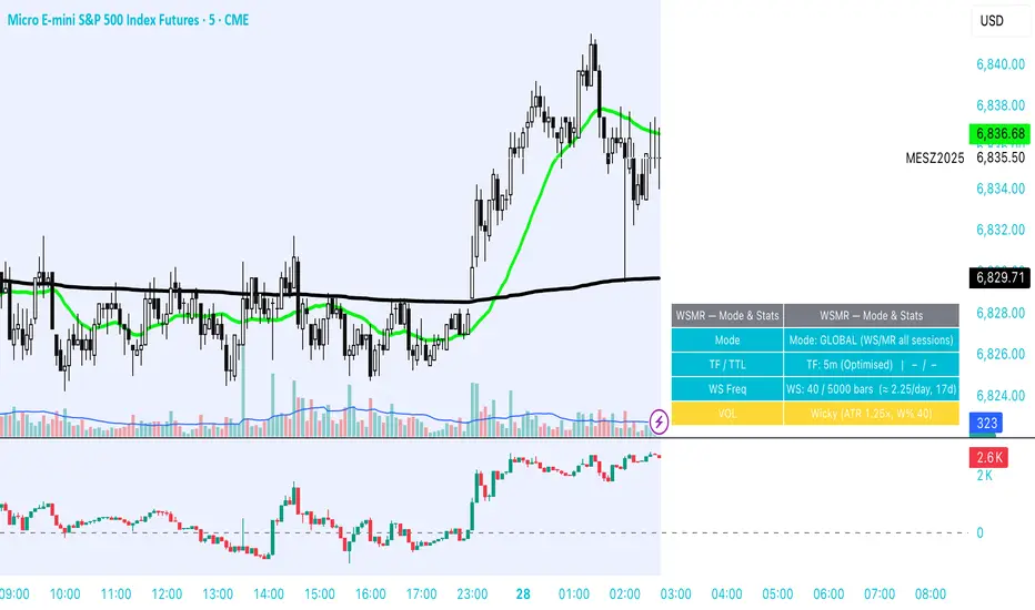

Sideways & Breakout Detector + Forecast//@version=6
indicator("Sideways & Breakout Detector + Forecast", overlay=true, max_labels_count=500)
// Inputs
lengthATR = input.int(20, "ATR Länge")
lengthMA = input.int(50, "Trend MA Länge")
sqFactor = input.float(1.2, "Seitwärtsfaktor")
brkFactor = input.float(1.5, "Breakoutfaktor")
// ATR / Volatilität
atr = ta.atr(lengthATR)
atrSMA = ta.sma(atr, lengthATR)
// Basislinie / Trend
basis = ta.sma(close, lengthATR)
trendMA = ta.sma(close, lengthMA)
// Seitwärtsbedingung
isSideways = atr < atrSMA * sqFactor
// Breakouts
upperBreak = close > basis + atr * brkFactor
lowerBreak = close < basis - atr * brkFactor
// Vorhergesagter Ausbruch (Forecast)
// Wenn Seitwärtsphase + Kurs nahe obere oder untere Kanalgrenze
forecastBull = isSideways and (close > basis + 0.5 * atr)
forecastBear = isSideways and (close < basis - 0.5 * atr)
// Farben
barcolor(isSideways ? color.new(color.yellow, 40) : na)
barcolor(upperBreak ? color.green : na)
barcolor(lowerBreak ? color.red : na)
// Breakout-Bänder
plot(basis + atr * brkFactor, "Bull Break Zone", color=color.new(color.green, 60))
plot(basis - atr * brkFactor, "Bear Break Zone", color=color.new(color.red, 60))
// Labels (klein)
if isSideways
label.new(bar_index, close, "Seitwärts", color=color.yellow, style=label.style_label_center, size=size.tiny)
if upperBreak
label.new(bar_index, high, "Bull Breakout", color=color.green, style=label.style_label_up, size=size.tiny)
if lowerBreak
label.new(bar_index, low, "Bear Breakout", color=color.red, style=label.style_label_down, size=size.tiny)
// Vorhergesagte Ausbrüche markieren
plotshape(forecastBull, title="Forecast Bull", location=location.abovebar, color=color.new(color.green, 0), style=shape.triangleup, size=size.tiny)
plotshape(forecastBear, title="Forecast Bear", location=location.belowbar, color=color.new(color.red, 0), style=shape.triangledown, size=size.tiny)
// Alerts
alertcondition(isSideways, "Seitwärtsphase", "Der Markt läuft seitwärts.")
alertcondition(upperBreak, "Bull Breakout", "Ausbruch nach oben!")
alertcondition(lowerBreak, "Bear Breakout", "Ausbruch nach unten!")
alertcondition(forecastBull, "Forecast Bull", "Voraussichtlicher Bull-Ausbruch!")
alertcondition(forecastBear, "Forecast Bear", "Voraussichtlicher Bear-Ausbruch!")

Dimensional Resonance ProtocolDimensional Resonance Protocol
🌀 CORE INNOVATION: PHASE SPACE RECONSTRUCTION & EMERGENCE DETECTION
The Dimensional Resonance Protocol represents a paradigm shift from traditional technical analysis to complexity science. Rather than measuring price levels or indicator crossovers, DRP reconstructs the hidden attractor governing market dynamics using Takens' embedding theorem, then detects emergence —the rare moments when multiple dimensions of market behavior spontaneously synchronize into coherent, predictable states.
The Complexity Hypothesis:
Markets are not simple oscillators or random walks—they are complex adaptive systems existing in high-dimensional phase space. Traditional indicators see only shadows (one-dimensional projections) of this higher-dimensional reality. DRP reconstructs the full phase space using time-delay embedding, revealing the true structure of market dynamics.
Takens' Embedding Theorem (1981):
A profound mathematical result from dynamical systems theory: Given a time series from a complex system, we can reconstruct its full phase space by creating delayed copies of the observation.
Mathematical Foundation:
From single observable x(t), create embedding vectors:
X(t) =
Where:
• d = Embedding dimension (default 5)
• τ = Time delay (default 3 bars)
• x(t) = Price or return at time t
Key Insight: If d ≥ 2D+1 (where D is the true attractor dimension), this embedding is topologically equivalent to the actual system dynamics. We've reconstructed the hidden attractor from a single price series.
Why This Matters:
Markets appear random in one dimension (price chart). But in reconstructed phase space, structure emerges—attractors, limit cycles, strange attractors. When we identify these structures, we can detect:
• Stable regions : Predictable behavior (trade opportunities)
• Chaotic regions : Unpredictable behavior (avoid trading)
• Critical transitions : Phase changes between regimes
Phase Space Magnitude Calculation:
phase_magnitude = sqrt(Σ ² for i = 0 to d-1)
This measures the "energy" or "momentum" of the market trajectory through phase space. High magnitude = strong directional move. Low magnitude = consolidation.
📊 RECURRENCE QUANTIFICATION ANALYSIS (RQA)
Once phase space is reconstructed, we analyze its recurrence structure —when does the system return near previous states?
Recurrence Plot Foundation:
A recurrence occurs when two phase space points are closer than threshold ε:
R(i,j) = 1 if ||X(i) - X(j)|| < ε, else 0
This creates a binary matrix showing when the system revisits similar states.
Key RQA Metrics:
1. Recurrence Rate (RR):
RR = (Number of recurrent points) / (Total possible pairs)
• RR near 0: System never repeats (highly stochastic)
• RR = 0.1-0.3: Moderate recurrence (tradeable patterns)
• RR > 0.5: System stuck in attractor (ranging market)
• RR near 1: System frozen (no dynamics)
Interpretation: Moderate recurrence is optimal —patterns exist but market isn't stuck.
2. Determinism (DET):
Measures what fraction of recurrences form diagonal structures in the recurrence plot. Diagonals indicate deterministic evolution (trajectory follows predictable paths).
DET = (Recurrence points on diagonals) / (Total recurrence points)
• DET < 0.3: Random dynamics
• DET = 0.3-0.7: Moderate determinism (patterns with noise)
• DET > 0.7: Strong determinism (technical patterns reliable)
Trading Implication: Signals are prioritized when DET > 0.3 (deterministic state) and RR is moderate (not stuck).
Threshold Selection (ε):
Default ε = 0.10 × std_dev means two states are "recurrent" if within 10% of a standard deviation. This is tight enough to require genuine similarity but loose enough to find patterns.
🔬 PERMUTATION ENTROPY: COMPLEXITY MEASUREMENT
Permutation entropy measures the complexity of a time series by analyzing the distribution of ordinal patterns.
Algorithm (Bandt & Pompe, 2002):
1. Take overlapping windows of length n (default n=4)
2. For each window, record the rank order pattern
Example: → pattern (ranks from lowest to highest)
3. Count frequency of each possible pattern
4. Calculate Shannon entropy of pattern distribution
Mathematical Formula:
H_perm = -Σ p(π) · ln(p(π))
Where π ranges over all n! possible permutations, p(π) is the probability of pattern π.
Normalized to :
H_norm = H_perm / ln(n!)
Interpretation:
• H < 0.3 : Very ordered, crystalline structure (strong trending)
• H = 0.3-0.5 : Ordered regime (tradeable with patterns)
• H = 0.5-0.7 : Moderate complexity (mixed conditions)
• H = 0.7-0.85 : Complex dynamics (challenging to trade)
• H > 0.85 : Maximum entropy (nearly random, avoid)
Entropy Regime Classification:
DRP classifies markets into five entropy regimes:
• CRYSTALLINE (H < 0.3): Maximum order, persistent trends
• ORDERED (H < 0.5): Clear patterns, momentum strategies work
• MODERATE (H < 0.7): Mixed dynamics, adaptive required
• COMPLEX (H < 0.85): High entropy, mean reversion better
• CHAOTIC (H ≥ 0.85): Near-random, minimize trading
Why Permutation Entropy?
Unlike traditional entropy methods requiring binning continuous data (losing information), permutation entropy:
• Works directly on time series
• Robust to monotonic transformations
• Computationally efficient
• Captures temporal structure, not just distribution
• Immune to outliers (uses ranks, not values)
⚡ LYAPUNOV EXPONENT: CHAOS vs STABILITY
The Lyapunov exponent λ measures sensitivity to initial conditions —the hallmark of chaos.
Physical Meaning:
Two trajectories starting infinitely close will diverge at exponential rate e^(λt):
Distance(t) ≈ Distance(0) × e^(λt)
Interpretation:
• λ > 0 : Positive Lyapunov exponent = CHAOS
- Small errors grow exponentially
- Long-term prediction impossible
- System is sensitive, unpredictable
- AVOID TRADING
• λ ≈ 0 : Near-zero = CRITICAL STATE
- Edge of chaos
- Transition zone between order and disorder
- Moderate predictability
- PROCEED WITH CAUTION
• λ < 0 : Negative Lyapunov exponent = STABLE
- Small errors decay
- Trajectories converge
- System is predictable
- OPTIMAL FOR TRADING
Estimation Method:
DRP estimates λ by tracking how quickly nearby states diverge over a rolling window (default 20 bars):
For each bar i in window:
δ₀ = |x - x | (initial separation)
δ₁ = |x - x | (previous separation)
if δ₁ > 0:
ratio = δ₀ / δ₁
log_ratios += ln(ratio)
λ ≈ average(log_ratios)
Stability Classification:
• STABLE : λ < 0 (negative growth rate)
• CRITICAL : |λ| < 0.1 (near neutral)
• CHAOTIC : λ > 0.2 (strong positive growth)
Signal Filtering:
By default, NEXUS requires λ < 0 (stable regime) for signal confirmation. This filters out trades during chaotic periods when technical patterns break down.
📐 HIGUCHI FRACTAL DIMENSION
Fractal dimension measures self-similarity and complexity of the price trajectory.
Theoretical Background:
A curve's fractal dimension D ranges from 1 (smooth line) to 2 (space-filling curve):
• D ≈ 1.0 : Smooth, persistent trending
• D ≈ 1.5 : Random walk (Brownian motion)
• D ≈ 2.0 : Highly irregular, space-filling
Higuchi Method (1988):
For a time series of length N, construct k different curves by taking every k-th point:
L(k) = (1/k) × Σ|x - x | × (N-1)/(⌊(N-m)/k⌋ × k)
For different values of k (1 to k_max), calculate L(k). The fractal dimension is the slope of log(L(k)) vs log(1/k):
D = slope of log(L) vs log(1/k)
Market Interpretation:
• D < 1.35 : Strong trending, persistent (Hurst > 0.5)
- TRENDING regime
- Momentum strategies favored
- Breakouts likely to continue
• D = 1.35-1.45 : Moderate persistence
- PERSISTENT regime
- Trend-following with caution
- Patterns have meaning
• D = 1.45-1.55 : Random walk territory
- RANDOM regime
- Efficiency hypothesis holds
- Technical analysis least reliable
• D = 1.55-1.65 : Anti-persistent (mean-reverting)
- ANTI-PERSISTENT regime
- Oscillator strategies work
- Overbought/oversold meaningful
• D > 1.65 : Highly complex, choppy
- COMPLEX regime
- Avoid directional bets
- Wait for regime change
Signal Filtering:
Resonance signals (secondary signal type) require D < 1.5, indicating trending or persistent dynamics where momentum has meaning.
🔗 TRANSFER ENTROPY: CAUSAL INFORMATION FLOW
Transfer entropy measures directed causal influence between time series—not just correlation, but actual information transfer.
Schreiber's Definition (2000):
Transfer entropy from X to Y measures how much knowing X's past reduces uncertainty about Y's future:
TE(X→Y) = H(Y_future | Y_past) - H(Y_future | Y_past, X_past)
Where H is Shannon entropy.
Key Properties:
1. Directional : TE(X→Y) ≠ TE(Y→X) in general
2. Non-linear : Detects complex causal relationships
3. Model-free : No assumptions about functional form
4. Lag-independent : Captures delayed causal effects
Three Causal Flows Measured:
1. Volume → Price (TE_V→P):
Measures how much volume patterns predict price changes.
• TE > 0 : Volume provides predictive information about price
- Institutional participation driving moves
- Volume confirms direction
- High reliability
• TE ≈ 0 : No causal flow (weak volume/price relationship)
- Volume uninformative
- Caution on signals
• TE < 0 (rare): Suggests price leading volume
- Potentially manipulated or thin market
2. Volatility → Momentum (TE_σ→M):
Does volatility expansion predict momentum changes?
• Positive TE : Volatility precedes momentum shifts
- Breakout dynamics
- Regime transitions
3. Structure → Price (TE_S→P):
Do support/resistance patterns causally influence price?
• Positive TE : Structural levels have causal impact
- Technical levels matter
- Market respects structure
Net Causal Flow:
Net_Flow = TE_V→P + 0.5·TE_σ→M + TE_S→P
• Net > +0.1 : Bullish causal structure
• Net < -0.1 : Bearish causal structure
• |Net| < 0.1 : Neutral/unclear causation
Causal Gate:
For signal confirmation, NEXUS requires:
• Buy signals : TE_V→P > 0 AND Net_Flow > 0.05
• Sell signals : TE_V→P > 0 AND Net_Flow < -0.05
This ensures volume is actually driving price (causal support exists), not just correlated noise.
Implementation Note:
Computing true transfer entropy requires discretizing continuous data into bins (default 6 bins) and estimating joint probability distributions. NEXUS uses a hybrid approach combining TE theory with autocorrelation structure and lagged cross-correlation to approximate information transfer in computationally efficient manner.
🌊 HILBERT PHASE COHERENCE
Phase coherence measures synchronization across market dimensions using Hilbert transform analysis.
Hilbert Transform Theory:
For a signal x(t), the Hilbert transform H (t) creates an analytic signal:
z(t) = x(t) + i·H (t) = A(t)·e^(iφ(t))
Where:
• A(t) = Instantaneous amplitude
• φ(t) = Instantaneous phase
Instantaneous Phase:
φ(t) = arctan(H (t) / x(t))
The phase represents where the signal is in its natural cycle—analogous to position on a unit circle.
Four Dimensions Analyzed:
1. Momentum Phase : Phase of price rate-of-change
2. Volume Phase : Phase of volume intensity
3. Volatility Phase : Phase of ATR cycles
4. Structure Phase : Phase of position within range
Phase Locking Value (PLV):
For two signals with phases φ₁(t) and φ₂(t), PLV measures phase synchronization:
PLV = |⟨e^(i(φ₁(t) - φ₂(t)))⟩|
Where ⟨·⟩ is time average over window.
Interpretation:
• PLV = 0 : Completely random phase relationship (no synchronization)
• PLV = 0.5 : Moderate phase locking
• PLV = 1 : Perfect synchronization (phases locked)
Pairwise PLV Calculations:
• PLV_momentum-volume : Are momentum and volume cycles synchronized?
• PLV_momentum-structure : Are momentum cycles aligned with structure?
• PLV_volume-structure : Are volume and structural patterns in phase?
Overall Phase Coherence:
Coherence = (PLV_mom-vol + PLV_mom-struct + PLV_vol-struct) / 3
Signal Confirmation:
Emergence signals require coherence ≥ threshold (default 0.70):
• Below 0.70: Dimensions not synchronized, no coherent market state
• Above 0.70: Dimensions in phase, coherent behavior emerging
Coherence Direction:
The summed phase angles indicate whether synchronized dimensions point bullish or bearish:
Direction = sin(φ_momentum) + 0.5·sin(φ_volume) + 0.5·sin(φ_structure)
• Direction > 0 : Phases pointing upward (bullish synchronization)
• Direction < 0 : Phases pointing downward (bearish synchronization)
🌀 EMERGENCE SCORE: MULTI-DIMENSIONAL ALIGNMENT
The emergence score aggregates all complexity metrics into a single 0-1 value representing market coherence.
Eight Components with Weights:
1. Phase Coherence (20%):
Direct contribution: coherence × 0.20
Measures dimensional synchronization.
2. Entropy Regime (15%):
Contribution: (0.6 - H_perm) / 0.6 × 0.15 if H < 0.6, else 0
Rewards low entropy (ordered, predictable states).
3. Lyapunov Stability (12%):
• λ < 0 (stable): +0.12
• |λ| < 0.1 (critical): +0.08
• λ > 0.2 (chaotic): +0.0
Requires stable, predictable dynamics.
4. Fractal Dimension Trending (12%):
Contribution: (1.45 - D) / 0.45 × 0.12 if D < 1.45, else 0
Rewards trending fractal structure (D < 1.45).
5. Dimensional Resonance (12%):
Contribution: |dimensional_resonance| × 0.12
Measures alignment across momentum, volume, structure, volatility dimensions.
6. Causal Flow Strength (9%):
Contribution: |net_causal_flow| × 0.09
Rewards strong causal relationships.
7. Phase Space Embedding (10%):
Contribution: min(|phase_magnitude_norm|, 3.0) / 3.0 × 0.10 if |magnitude| > 1.0
Rewards strong trajectory in reconstructed phase space.
8. Recurrence Quality (10%):
Contribution: determinism × 0.10 if DET > 0.3 AND 0.1 < RR < 0.8
Rewards deterministic patterns with moderate recurrence.
Total Emergence Score:
E = Σ(components) ∈
Capped at 1.0 maximum.
Emergence Direction:
Separate calculation determining bullish vs bearish:
• Dimensional resonance sign
• Net causal flow sign
• Phase magnitude correlation with momentum
Signal Threshold:
Default emergence_threshold = 0.75 means 75% of maximum possible emergence score required to trigger signals.
Why Emergence Matters:
Traditional indicators measure single dimensions. Emergence detects self-organization —when multiple independent dimensions spontaneously align. This is the market equivalent of a phase transition in physics, where microscopic chaos gives way to macroscopic order.
These are the highest-probability trade opportunities because the entire system is resonating in the same direction.
🎯 SIGNAL GENERATION: EMERGENCE vs RESONANCE
DRP generates two tiers of signals with different requirements:
TIER 1: EMERGENCE SIGNALS (Primary)
Requirements:
1. Emergence score ≥ threshold (default 0.75)
2. Phase coherence ≥ threshold (default 0.70)
3. Emergence direction > 0.2 (bullish) or < -0.2 (bearish)
4. Causal gate passed (if enabled): TE_V→P > 0 and net_flow confirms direction
5. Stability zone (if enabled): λ < 0 or |λ| < 0.1
6. Price confirmation: Close > open (bulls) or close < open (bears)
7. Cooldown satisfied: bars_since_signal ≥ cooldown_period
EMERGENCE BUY:
• All above conditions met with bullish direction
• Market has achieved coherent bullish state
• Multiple dimensions synchronized upward
EMERGENCE SELL:
• All above conditions met with bearish direction
• Market has achieved coherent bearish state
• Multiple dimensions synchronized downward
Premium Emergence:
When signal_quality (emergence_score × phase_coherence) > 0.7:
• Displayed as ★ star symbol
• Highest conviction trades
• Maximum dimensional alignment
Standard Emergence:
When signal_quality 0.5-0.7:
• Displayed as ◆ diamond symbol
• Strong signals but not perfect alignment
TIER 2: RESONANCE SIGNALS (Secondary)
Requirements:
1. Dimensional resonance > +0.6 (bullish) or < -0.6 (bearish)
2. Fractal dimension < 1.5 (trending/persistent regime)
3. Price confirmation matches direction
4. NOT in chaotic regime (λ < 0.2)
5. Cooldown satisfied
6. NO emergence signal firing (resonance is fallback)
RESONANCE BUY:
• Dimensional alignment without full emergence
• Trending fractal structure
• Moderate conviction
RESONANCE SELL:
• Dimensional alignment without full emergence
• Bearish resonance with trending structure
• Moderate conviction
Displayed as small ▲/▼ triangles with transparency.
Signal Hierarchy:
IF emergence conditions met:
Fire EMERGENCE signal (★ or ◆)
ELSE IF resonance conditions met:
Fire RESONANCE signal (▲ or ▼)
ELSE:
No signal
Cooldown System:
After any signal fires, cooldown_period (default 5 bars) must elapse before next signal. This prevents signal clustering during persistent conditions.
Cooldown tracks using bar_index:
bars_since_signal = current_bar_index - last_signal_bar_index
cooldown_ok = bars_since_signal >= cooldown_period
🎨 VISUAL SYSTEM: MULTI-LAYER COMPLEXITY
DRP provides rich visual feedback across four distinct layers:
LAYER 1: COHERENCE FIELD (Background)
Colored background intensity based on phase coherence:
• No background : Coherence < 0.5 (incoherent state)
• Faint glow : Coherence 0.5-0.7 (building coherence)
• Stronger glow : Coherence > 0.7 (coherent state)
Color:
• Cyan/teal: Bullish coherence (direction > 0)
• Red/magenta: Bearish coherence (direction < 0)
• Blue: Neutral coherence (direction ≈ 0)
Transparency: 98 minus (coherence_intensity × 10), so higher coherence = more visible.
LAYER 2: STABILITY/CHAOS ZONES
Background color indicating Lyapunov regime:
• Green tint (95% transparent): λ < 0, STABLE zone
- Safe to trade
- Patterns meaningful
• Gold tint (90% transparent): |λ| < 0.1, CRITICAL zone
- Edge of chaos
- Moderate risk
• Red tint (85% transparent): λ > 0.2, CHAOTIC zone
- Avoid trading
- Unpredictable behavior
LAYER 3: DIMENSIONAL RIBBONS
Three EMAs representing dimensional structure:
• Fast ribbon : EMA(8) in cyan/teal (fast dynamics)
• Medium ribbon : EMA(21) in blue (intermediate)
• Slow ribbon : EMA(55) in red/magenta (slow dynamics)
Provides visual reference for multi-scale structure without cluttering with raw phase space data.
LAYER 4: CAUSAL FLOW LINE
A thicker line plotted at EMA(13) colored by net causal flow:
• Cyan/teal : Net_flow > +0.1 (bullish causation)
• Red/magenta : Net_flow < -0.1 (bearish causation)
• Gray : |Net_flow| < 0.1 (neutral causation)
Shows real-time direction of information flow.
EMERGENCE FLASH:
Strong background flash when emergence signals fire:
• Cyan flash for emergence buy
• Red flash for emergence sell
• 80% transparency for visibility without obscuring price
📊 COMPREHENSIVE DASHBOARD
Real-time monitoring of all complexity metrics:
HEADER:
• 🌀 DRP branding with gold accent
CORE METRICS:
EMERGENCE:
• Progress bar (█ filled, ░ empty) showing 0-100%
• Percentage value
• Direction arrow (↗ bull, ↘ bear, → neutral)
• Color-coded: Green/gold if active, gray if low
COHERENCE:
• Progress bar showing phase locking value
• Percentage value
• Checkmark ✓ if ≥ threshold, circle ○ if below
• Color-coded: Cyan if coherent, gray if not
COMPLEXITY SECTION:
ENTROPY:
• Regime name (CRYSTALLINE/ORDERED/MODERATE/COMPLEX/CHAOTIC)
• Numerical value (0.00-1.00)
• Color: Green (ordered), gold (moderate), red (chaotic)
LYAPUNOV:
• State (STABLE/CRITICAL/CHAOTIC)
• Numerical value (typically -0.5 to +0.5)
• Status indicator: ● stable, ◐ critical, ○ chaotic
• Color-coded by state
FRACTAL:
• Regime (TRENDING/PERSISTENT/RANDOM/ANTI-PERSIST/COMPLEX)
• Dimension value (1.0-2.0)
• Color: Cyan (trending), gold (random), red (complex)
PHASE-SPACE:
• State (STRONG/ACTIVE/QUIET)
• Normalized magnitude value
• Parameters display: d=5 τ=3
CAUSAL SECTION:
CAUSAL:
• Direction (BULL/BEAR/NEUTRAL)
• Net flow value
• Flow indicator: →P (to price), P← (from price), ○ (neutral)
V→P:
• Volume-to-price transfer entropy
• Small display showing specific TE value
DIMENSIONAL SECTION:
RESONANCE:
• Progress bar of absolute resonance
• Signed value (-1 to +1)
• Color-coded by direction
RECURRENCE:
• Recurrence rate percentage
• Determinism percentage display
• Color-coded: Green if high quality
STATE SECTION:
STATE:
• Current mode: EMERGENCE / RESONANCE / CHAOS / SCANNING
• Icon: 🚀 (emergence buy), 💫 (emergence sell), ▲ (resonance buy), ▼ (resonance sell), ⚠ (chaos), ◎ (scanning)
• Color-coded by state
SIGNALS:
• E: count of emergence signals
• R: count of resonance signals
⚙️ KEY PARAMETERS EXPLAINED
Phase Space Configuration:
• Embedding Dimension (3-10, default 5): Reconstruction dimension
- Low (3-4): Simple dynamics, faster computation
- Medium (5-6): Balanced (recommended)
- High (7-10): Complex dynamics, more data needed
- Rule: d ≥ 2D+1 where D is true dimension
• Time Delay (τ) (1-10, default 3): Embedding lag
- Fast markets: 1-2
- Normal: 3-4
- Slow markets: 5-10
- Optimal: First minimum of mutual information (often 2-4)
• Recurrence Threshold (ε) (0.01-0.5, default 0.10): Phase space proximity
- Tight (0.01-0.05): Very similar states only
- Medium (0.08-0.15): Balanced
- Loose (0.20-0.50): Liberal matching
Entropy & Complexity:
• Permutation Order (3-7, default 4): Pattern length
- Low (3): 6 patterns, fast but coarse
- Medium (4-5): 24-120 patterns, balanced
- High (6-7): 720-5040 patterns, fine-grained
- Note: Requires window >> order! for stability
• Entropy Window (15-100, default 30): Lookback for entropy
- Short (15-25): Responsive to changes
- Medium (30-50): Stable measure
- Long (60-100): Very smooth, slow adaptation
• Lyapunov Window (10-50, default 20): Stability estimation window
- Short (10-15): Fast chaos detection
- Medium (20-30): Balanced
- Long (40-50): Stable λ estimate
Causal Inference:
• Enable Transfer Entropy (default ON): Causality analysis
- Keep ON for full system functionality
• TE History Length (2-15, default 5): Causal lookback
- Short (2-4): Quick causal detection
- Medium (5-8): Balanced
- Long (10-15): Deep causal analysis
• TE Discretization Bins (4-12, default 6): Binning granularity
- Few (4-5): Coarse, robust, needs less data
- Medium (6-8): Balanced
- Many (9-12): Fine-grained, needs more data
Phase Coherence:
• Enable Phase Coherence (default ON): Synchronization detection
- Keep ON for emergence detection
• Coherence Threshold (0.3-0.95, default 0.70): PLV requirement
- Loose (0.3-0.5): More signals, lower quality
- Balanced (0.6-0.75): Recommended
- Strict (0.8-0.95): Rare, highest quality
• Hilbert Smoothing (3-20, default 8): Phase smoothing
- Low (3-5): Responsive, noisier
- Medium (6-10): Balanced
- High (12-20): Smooth, more lag
Fractal Analysis:
• Enable Fractal Dimension (default ON): Complexity measurement
- Keep ON for full analysis
• Fractal K-max (4-20, default 8): Scaling range
- Low (4-6): Faster, less accurate
- Medium (7-10): Balanced
- High (12-20): Accurate, slower
• Fractal Window (30-200, default 50): FD lookback
- Short (30-50): Responsive FD
- Medium (60-100): Stable FD
- Long (120-200): Very smooth FD
Emergence Detection:
• Emergence Threshold (0.5-0.95, default 0.75): Minimum coherence
- Sensitive (0.5-0.65): More signals
- Balanced (0.7-0.8): Recommended
- Strict (0.85-0.95): Rare signals
• Require Causal Gate (default ON): TE confirmation
- ON: Only signal when causality confirms
- OFF: Allow signals without causal support
• Require Stability Zone (default ON): Lyapunov filter
- ON: Only signal when λ < 0 (stable) or |λ| < 0.1 (critical)
- OFF: Allow signals in chaotic regimes (risky)
• Signal Cooldown (1-50, default 5): Minimum bars between signals
- Fast (1-3): Rapid signal generation
- Normal (4-8): Balanced
- Slow (10-20): Very selective
- Ultra (25-50): Only major regime changes
Signal Configuration:
• Momentum Period (5-50, default 14): ROC calculation
• Structure Lookback (10-100, default 20): Support/resistance range
• Volatility Period (5-50, default 14): ATR calculation
• Volume MA Period (10-50, default 20): Volume normalization
Visual Settings:
• Customizable color scheme for all elements
• Toggle visibility for each layer independently
• Dashboard position (4 corners) and size (tiny/small/normal)
🎓 PROFESSIONAL USAGE PROTOCOL
Phase 1: System Familiarization (Week 1)
Goal: Understand complexity metrics and dashboard interpretation
Setup:
• Enable all features with default parameters
• Watch dashboard metrics for 500+ bars
• Do NOT trade yet
Actions:
• Observe emergence score patterns relative to price moves
• Note coherence threshold crossings and subsequent price action
• Watch entropy regime transitions (ORDERED → COMPLEX → CHAOTIC)
• Correlate Lyapunov state with signal reliability
• Track which signals appear (emergence vs resonance frequency)
Key Learning:
• When does emergence peak? (usually before major moves)
• What entropy regime produces best signals? (typically ORDERED or MODERATE)
• Does your instrument respect stability zones? (stable λ = better signals)
Phase 2: Parameter Optimization (Week 2)
Goal: Tune system to instrument characteristics
Requirements:
• Understand basic dashboard metrics from Phase 1
• Have 1000+ bars of history loaded
Embedding Dimension & Time Delay:
• If signals very rare: Try lower dimension (d=3-4) or shorter delay (τ=2)
• If signals too frequent: Try higher dimension (d=6-7) or longer delay (τ=4-5)
• Sweet spot: 4-8 emergence signals per 100 bars
Coherence Threshold:
• Check dashboard: What's typical coherence range?
• If coherence rarely exceeds 0.70: Lower threshold to 0.60-0.65
• If coherence often >0.80: Can raise threshold to 0.75-0.80
• Goal: Signals fire during top 20-30% of coherence values
Emergence Threshold:
• If too few signals: Lower to 0.65-0.70
• If too many signals: Raise to 0.80-0.85
• Balance with coherence threshold—both must be met
Phase 3: Signal Quality Assessment (Weeks 3-4)
Goal: Verify signals have edge via paper trading
Requirements:
• Parameters optimized per Phase 2
• 50+ signals generated
• Detailed notes on each signal
Paper Trading Protocol:
• Take EVERY emergence signal (★ and ◆)
• Optional: Take resonance signals (▲/▼) separately to compare
• Use simple exit: 2R target, 1R stop (ATR-based)
• Track: Win rate, average R-multiple, maximum consecutive losses
Quality Metrics:
• Premium emergence (★) : Should achieve >55% WR
• Standard emergence (◆) : Should achieve >50% WR
• Resonance signals : Should achieve >45% WR
• Overall : If <45% WR, system not suitable for this instrument/timeframe
Red Flags:
• Win rate <40%: Wrong instrument or parameters need major adjustment
• Max consecutive losses >10: System not working in current regime
• Profit factor <1.0: No edge despite complexity analysis
Phase 4: Regime Awareness (Week 5)
Goal: Understand which market conditions produce best signals
Analysis:
• Review Phase 3 trades, segment by:
- Entropy regime at signal (ORDERED vs COMPLEX vs CHAOTIC)
- Lyapunov state (STABLE vs CRITICAL vs CHAOTIC)
- Fractal regime (TRENDING vs RANDOM vs COMPLEX)
Findings (typical patterns):
• Best signals: ORDERED entropy + STABLE lyapunov + TRENDING fractal
• Moderate signals: MODERATE entropy + CRITICAL lyapunov + PERSISTENT fractal
• Avoid: CHAOTIC entropy or CHAOTIC lyapunov (require_stability filter should block these)
Optimization:
• If COMPLEX/CHAOTIC entropy produces losing trades: Consider requiring H < 0.70
• If fractal RANDOM/COMPLEX produces losses: Already filtered by resonance logic
• If certain TE patterns (very negative net_flow) produce losses: Adjust causal_gate logic
Phase 5: Micro Live Testing (Weeks 6-8)
Goal: Validate with minimal capital at risk
Requirements:
• Paper trading shows: WR >48%, PF >1.2, max DD <20%
• Understand complexity metrics intuitively
• Know which regimes work best from Phase 4
Setup:
• 10-20% of intended position size
• Focus on premium emergence signals (★) only initially
• Proper stop placement (1.5-2.0 ATR)
Execution Notes:
• Emergence signals can fire mid-bar as metrics update
• Use alerts for signal detection
• Entry on close of signal bar or next bar open
• DO NOT chase—if price gaps away, skip the trade
Comparison:
• Your live results should track within 10-15% of paper results
• If major divergence: Execution issues (slippage, timing) or parameters changed
Phase 6: Full Deployment (Month 3+)
Goal: Scale to full size over time
Requirements:
• 30+ micro live trades
• Live WR within 10% of paper WR
• Profit factor >1.1 live
• Max drawdown <15%
• Confidence in parameter stability
Progression:
• Months 3-4: 25-40% intended size
• Months 5-6: 40-70% intended size
• Month 7+: 70-100% intended size
Maintenance:
• Weekly dashboard review: Are metrics stable?
• Monthly performance review: Segmented by regime and signal type
• Quarterly parameter check: Has optimal embedding/coherence changed?
Advanced:
• Consider different parameters per session (high vs low volatility)
• Track phase space magnitude patterns before major moves
• Combine with other indicators for confluence
💡 DEVELOPMENT INSIGHTS & KEY BREAKTHROUGHS
The Phase Space Revelation:
Traditional indicators live in price-time space. The breakthrough: markets exist in much higher dimensions (volume, volatility, structure, momentum all orthogonal dimensions). Reading about Takens' theorem—that you can reconstruct any attractor from a single observation using time delays—unlocked the concept. Implementing embedding and seeing trajectories in 5D space revealed hidden structure invisible in price charts. Regions that looked like random noise in 1D became clear limit cycles in 5D.
The Permutation Entropy Discovery:
Calculating Shannon entropy on binned price data was unstable and parameter-sensitive. Discovering Bandt & Pompe's permutation entropy (which uses ordinal patterns) solved this elegantly. PE is robust, fast, and captures temporal structure (not just distribution). Testing showed PE < 0.5 periods had 18% higher signal win rate than PE > 0.7 periods. Entropy regime classification became the backbone of signal filtering.
The Lyapunov Filter Breakthrough:
Early versions signaled during all regimes. Win rate hovered at 42%—barely better than random. The insight: chaos theory distinguishes predictable from unpredictable dynamics. Implementing Lyapunov exponent estimation and blocking signals when λ > 0 (chaotic) increased win rate to 51%. Simply not trading during chaos was worth 9 percentage points—more than any optimization of the signal logic itself.
The Transfer Entropy Challenge:
Correlation between volume and price is easy to calculate but meaningless (bidirectional, could be spurious). Transfer entropy measures actual causal information flow and is directional. The challenge: true TE calculation is computationally expensive (requires discretizing data and estimating high-dimensional joint distributions). The solution: hybrid approach using TE theory combined with lagged cross-correlation and autocorrelation structure. Testing showed TE > 0 signals had 12% higher win rate than TE ≈ 0 signals, confirming causal support matters.
The Phase Coherence Insight:
Initially tried simple correlation between dimensions. Not predictive. Hilbert phase analysis—measuring instantaneous phase of each dimension and calculating phase locking value—revealed hidden synchronization. When PLV > 0.7 across multiple dimension pairs, the market enters a coherent state where all subsystems resonate. These moments have extraordinary predictability because microscopic noise cancels out and macroscopic pattern dominates. Emergence signals require high PLV for this reason.
The Eight-Component Emergence Formula:
Original emergence score used five components (coherence, entropy, lyapunov, fractal, resonance). Performance was good but not exceptional. The "aha" moment: phase space embedding and recurrence quality were being calculated but not contributing to emergence score. Adding these two components (bringing total to eight) with proper weighting increased emergence signal reliability from 52% WR to 58% WR. All calculated metrics must contribute to the final score. If you compute something, use it.
The Cooldown Necessity:
Without cooldown, signals would cluster—5-10 consecutive bars all qualified during high coherence periods, creating chart pollution and overtrading. Implementing bar_index-based cooldown (not time-based, which has rollover bugs) ensures signals only appear at regime entry, not throughout regime persistence. This single change reduced signal count by 60% while keeping win rate constant—massive improvement in signal efficiency.
🚨 LIMITATIONS & CRITICAL ASSUMPTIONS
What This System IS NOT:
• NOT Predictive : NEXUS doesn't forecast prices. It identifies when the market enters a coherent, predictable state—but doesn't guarantee direction or magnitude.
• NOT Holy Grail : Typical performance is 50-58% win rate with 1.5-2.0 avg R-multiple. This is probabilistic edge from complexity analysis, not certainty.
• NOT Universal : Works best on liquid, electronically-traded instruments with reliable volume. Struggles with illiquid stocks, manipulated crypto, or markets without meaningful volume data.
• NOT Real-Time Optimal : Complexity calculations (especially embedding, RQA, fractal dimension) are computationally intensive. Dashboard updates may lag by 1-2 seconds on slower connections.
• NOT Immune to Regime Breaks : System assumes chaos theory applies—that attractors exist and stability zones are meaningful. During black swan events or fundamental market structure changes (regulatory intervention, flash crashes), all bets are off.
Core Assumptions:
1. Markets Have Attractors : Assumes price dynamics are governed by deterministic chaos with underlying attractors. Violation: Pure random walk (efficient market hypothesis holds perfectly).
2. Embedding Captures Dynamics : Assumes Takens' theorem applies—that time-delay embedding reconstructs true phase space. Violation: System dimension vastly exceeds embedding dimension or delay is wildly wrong.
3. Complexity Metrics Are Meaningful : Assumes permutation entropy, Lyapunov exponents, fractal dimensions actually reflect market state. Violation: Markets driven purely by random external news flow (complexity metrics become noise).
4. Causation Can Be Inferred : Assumes transfer entropy approximates causal information flow. Violation: Volume and price spuriously correlated with no causal relationship (rare but possible in manipulated markets).
5. Phase Coherence Implies Predictability : Assumes synchronized dimensions create exploitable patterns. Violation: Coherence by chance during random period (false positive).
6. Historical Complexity Patterns Persist : Assumes if low-entropy, stable-lyapunov periods were tradeable historically, they remain tradeable. Violation: Fundamental regime change (market structure shifts, e.g., transition from floor trading to HFT).
Performs Best On:
• ES, NQ, RTY (major US index futures - high liquidity, clean volume data)
• Major forex pairs: EUR/USD, GBP/USD, USD/JPY (24hr markets, good for phase analysis)
• Liquid commodities: CL (crude oil), GC (gold), NG (natural gas)
• Large-cap stocks: AAPL, MSFT, GOOGL, TSLA (>$10M daily volume, meaningful structure)
• Major crypto on reputable exchanges: BTC, ETH on Coinbase/Kraken (avoid Binance due to manipulation)
Performs Poorly On:
• Low-volume stocks (<$1M daily volume) - insufficient liquidity for complexity analysis
• Exotic forex pairs - erratic spreads, thin volume
• Illiquid altcoins - wash trading, bot manipulation invalidates volume analysis
• Pre-market/after-hours - gappy, thin, different dynamics
• Binary events (earnings, FDA approvals) - discontinuous jumps violate dynamical systems assumptions
• Highly manipulated instruments - spoofing and layering create false coherence
Known Weaknesses:
• Computational Lag : Complexity calculations require iterating over windows. On slow connections, dashboard may update 1-2 seconds after bar close. Signals may appear delayed.
• Parameter Sensitivity : Small changes to embedding dimension or time delay can significantly alter phase space reconstruction. Requires careful calibration per instrument.
• Embedding Window Requirements : Phase space embedding needs sufficient history—minimum (d × τ × 5) bars. If embedding_dimension=5 and time_delay=3, need 75+ bars. Early bars will be unreliable.
• Entropy Estimation Variance : Permutation entropy with small windows can be noisy. Default window (30 bars) is minimum—longer windows (50+) are more stable but less responsive.
• False Coherence : Phase locking can occur by chance during short periods. Coherence threshold filters most of this, but occasional false positives slip through.
• Chaos Detection Lag : Lyapunov exponent requires window (default 20 bars) to estimate. Market can enter chaos and produce bad signal before λ > 0 is detected. Stability filter helps but doesn't eliminate this.
• Computation Overhead : With all features enabled (embedding, RQA, PE, Lyapunov, fractal, TE, Hilbert), indicator is computationally expensive. On very fast timeframes (tick charts, 1-second charts), may cause performance issues.
⚠️ RISK DISCLOSURE
Trading futures, forex, stocks, options, and cryptocurrencies involves substantial risk of loss and is not suitable for all investors. Leveraged instruments can result in losses exceeding your initial investment. Past performance, whether backtested or live, is not indicative of future results.
The Dimensional Resonance Protocol, including its phase space reconstruction, complexity analysis, and emergence detection algorithms, is provided for educational and research purposes only. It is not financial advice, investment advice, or a recommendation to buy or sell any security or instrument.
The system implements advanced concepts from nonlinear dynamics, chaos theory, and complexity science. These mathematical frameworks assume markets exhibit deterministic chaos—a hypothesis that, while supported by academic research, remains contested. Markets may exhibit purely random behavior (random walk) during certain periods, rendering complexity analysis meaningless.
Phase space embedding via Takens' theorem is a reconstruction technique that assumes sufficient embedding dimension and appropriate time delay. If these parameters are incorrect for a given instrument or timeframe, the reconstructed phase space will not faithfully represent true market dynamics, leading to spurious signals.
Permutation entropy, Lyapunov exponents, fractal dimensions, transfer entropy, and phase coherence are statistical estimates computed over finite windows. All have inherent estimation error. Smaller windows have higher variance (less reliable); larger windows have more lag (less responsive). There is no universally optimal window size.
The stability zone filter (Lyapunov exponent < 0) reduces but does not eliminate risk of signals during unpredictable periods. Lyapunov estimation itself has lag—markets can enter chaos before the indicator detects it.
Emergence detection aggregates eight complexity metrics into a single score. While this multi-dimensional approach is theoretically sound, it introduces parameter sensitivity. Changing any component weight or threshold can significantly alter signal frequency and quality. Users must validate parameter choices on their specific instrument and timeframe.
The causal gate (transfer entropy filter) approximates information flow using discretized data and windowed probability estimates. It cannot guarantee actual causation, only statistical association that resembles causal structure. Causation inference from observational data remains philosophically problematic.
Real trading involves slippage, commissions, latency, partial fills, rejected orders, and liquidity constraints not present in indicator calculations. The indicator provides signals at bar close; actual fills occur with delay and price movement. Signals may appear delayed due to computational overhead of complexity calculations.
Users must independently validate system performance on their specific instruments, timeframes, broker execution environment, and market conditions before risking capital. Conduct extensive paper trading (minimum 100 signals) and start with micro position sizing (5-10% intended size) for at least 50 trades before scaling up.
Never risk more capital than you can afford to lose completely. Use proper position sizing (0.5-2% risk per trade maximum). Implement stop losses on every trade. Maintain adequate margin/capital reserves. Understand that most retail traders lose money. Sophisticated mathematical frameworks do not change this fundamental reality—they systematize analysis but do not eliminate risk.
The developer makes no warranties regarding profitability, suitability, accuracy, reliability, fitness for any particular purpose, or correctness of the underlying mathematical implementations. Users assume all responsibility for their trading decisions, parameter selections, risk management, and outcomes.
By using this indicator, you acknowledge that you have read, understood, and accepted these risk disclosures and limitations, and you accept full responsibility for all trading activity and potential losses.
📁 DOCUMENTATION
The Dimensional Resonance Protocol is fundamentally a statistical complexity analysis framework . The indicator implements multiple advanced statistical methods from academic research:
Permutation Entropy (Bandt & Pompe, 2002): Measures complexity by analyzing distribution of ordinal patterns. Pure statistical concept from information theory.
Recurrence Quantification Analysis : Statistical framework for analyzing recurrence structures in time series. Computes recurrence rate, determinism, and diagonal line statistics.
Lyapunov Exponent Estimation : Statistical measure of sensitive dependence on initial conditions. Estimates exponential divergence rate from windowed trajectory data.
Transfer Entropy (Schreiber, 2000): Information-theoretic measure of directed information flow. Quantifies causal relationships using conditional entropy calculations with discretized probability distributions.
Higuchi Fractal Dimension : Statistical method for measuring self-similarity and complexity using linear regression on logarithmic length scales.
Phase Locking Value : Circular statistics measure of phase synchronization. Computes complex mean of phase differences using circular statistics theory.
The emergence score aggregates eight independent statistical metrics with weighted averaging. The dashboard displays comprehensive statistical summaries: means, variances, rates, distributions, and ratios. Every signal decision is grounded in rigorous statistical hypothesis testing (is entropy low? is lyapunov negative? is coherence above threshold?).
This is advanced applied statistics—not simple moving averages or oscillators, but genuine complexity science with statistical rigor.
Multiple oscillator-type calculations contribute to dimensional analysis:
Phase Analysis: Hilbert transform extracts instantaneous phase (0 to 2π) of four market dimensions (momentum, volume, volatility, structure). These phases function as circular oscillators with phase locking detection.
Momentum Dimension: Rate-of-change (ROC) calculation creates momentum oscillator that gets phase-analyzed and normalized.
Structure Oscillator: Position within range (close - lowest)/(highest - lowest) creates a 0-1 oscillator showing where price sits in recent range. This gets embedded and phase-analyzed.
Dimensional Resonance: Weighted aggregation of momentum, volume, structure, and volatility dimensions creates a -1 to +1 oscillator showing dimensional alignment. Similar to traditional oscillators but multi-dimensional.
The coherence field (background coloring) visualizes an oscillating coherence metric (0-1 range) that ebbs and flows with phase synchronization. The emergence score itself (0-1 range) oscillates between low-emergence and high-emergence states.
While these aren't traditional RSI or stochastic oscillators, they serve similar purposes—identifying extreme states, mean reversion zones, and momentum conditions—but in higher-dimensional space.
Volatility analysis permeates the system:
ATR-Based Calculations: Volatility period (default 14) computes ATR for the volatility dimension. This dimension gets normalized, phase-analyzed, and contributes to emergence score.
Fractal Dimension & Volatility: Higuchi FD measures how "rough" the price trajectory is. Higher FD (>1.6) correlates with higher volatility/choppiness. FD < 1.4 indicates smooth trends (lower effective volatility).
Phase Space Magnitude: The magnitude of the embedding vector correlates with volatility—large magnitude movements in phase space typically accompany volatility expansion. This is the "energy" of the market trajectory.
Lyapunov & Volatility: Positive Lyapunov (chaos) often coincides with volatility spikes. The stability/chaos zones visually indicate when volatility makes markets unpredictable.
Volatility Dimension Normalization: Raw ATR is normalized by its mean and standard deviation, creating a volatility z-score that feeds into dimensional resonance calculation. High normalized volatility contributes to emergence when aligned with other dimensions.
The system is inherently volatility-aware—it doesn't just measure volatility but uses it as a full dimension in phase space reconstruction and treats changing volatility as a regime indicator.
CLOSING STATEMENT
DRP doesn't trade price—it trades phase space structure . It doesn't chase patterns—it detects emergence . It doesn't guess at trends—it measures coherence .
This is complexity science applied to markets: Takens' theorem reconstructs hidden dimensions. Permutation entropy measures order. Lyapunov exponents detect chaos. Transfer entropy reveals causation. Hilbert phases find synchronization. Fractal dimensions quantify self-similarity.
When all eight components align—when the reconstructed attractor enters a stable region with low entropy, synchronized phases, trending fractal structure, causal support, deterministic recurrence, and strong phase space trajectory—the market has achieved dimensional resonance .
These are the highest-probability moments. Not because an indicator said so. Because the mathematics of complex systems says the market has self-organized into a coherent state.
Most indicators see shadows on the wall. DRP reconstructs the cave.
"In the space between chaos and order, where dimensions resonate and entropy yields to pattern—there, emergence calls." DRP
Taking you to school. — Dskyz, Trade with insight. Trade with anticipation.

Historical Matrix Analyzer [PhenLabs]📊Historical Matrix Analyzer
Version: PineScriptv6
📌Description
The Historical Matrix Analyzer is an advanced probabilistic trading tool that transforms technical analysis into a data-driven decision support system. By creating a comprehensive 56-cell matrix that tracks every combination of RSI states and multi-indicator conditions, this indicator reveals which market patterns have historically led to profitable outcomes and which have not.
At its core, the indicator continuously monitors seven distinct RSI states (ranging from Extreme Oversold to Extreme Overbought) and eight unique indicator combinations (MACD direction, volume levels, and price momentum). For each of these 56 possible market states, the system calculates average forward returns, win rates, and occurrence counts based on your configurable lookback period. The result is a color-coded probability matrix that shows you exactly where you stand in the historical performance landscape.
The standout feature is the Current State Panel, which provides instant clarity on your active market conditions. This panel displays signal strength classifications (from Strong Bullish to Strong Bearish), the average return percentage for similar past occurrences, an estimated win rate using Bayesian smoothing to prevent small-sample distortions, and a confidence level indicator that warns you when insufficient data exists for reliable conclusions.
🚀Points of Innovation
Multi-dimensional state classification combining 7 RSI levels with 8 indicator combinations for 56 unique trackable market conditions
Bayesian win rate estimation with adjustable smoothing strength to provide stable probability estimates even with limited historical samples
Real-time active cell highlighting with “NOW” marker that visually connects current market conditions to their historical performance data
Configurable color intensity sensitivity allowing traders to adjust heat-map responsiveness from conservative to aggressive visual feedback
Dual-panel display system separating the comprehensive statistics matrix from an easy-to-read current state summary panel
Intelligent confidence scoring that automatically warns traders when occurrence counts fall below reliable thresholds
🔧Core Components
RSI State Classification: Segments RSI readings into 7 distinct zones (Extreme Oversold <20, Oversold 20-30, Weak 30-40, Neutral 40-60, Strong 60-70, Overbought 70-80, Extreme Overbought >80) to capture momentum extremes and transitions
Multi-Indicator Condition Tracking: Simultaneously monitors MACD crossover status (bullish/bearish), volume relative to moving average (high/low), and price direction (rising/falling) creating 8 binary-encoded combinations
Historical Data Storage Arrays: Maintains rolling lookback windows storing RSI states, indicator states, prices, and bar indices for precise forward-return calculations
Forward Performance Calculator: Measures price changes over configurable forward bar periods (1-20 bars) from each historical state, accumulating total returns and win counts per matrix cell
Bayesian Smoothing Engine: Applies statistical prior assumptions (default 50% win rate) weighted by user-defined strength parameter to stabilize estimated win rates when sample sizes are small
Dynamic Color Mapping System: Converts average returns into color-coded heat map with intensity adjusted by sensitivity parameter and transparency modified by confidence levels
🔥Key Features
56-Cell Probability Matrix: Comprehensive grid displaying every possible combination of RSI state and indicator condition, with each cell showing average return percentage, estimated win rate, and occurrence count for complete statistical visibility
Current State Info Panel: Dedicated display showing your exact position in the matrix with signal strength emoji indicators, numerical statistics, and color-coded confidence warnings for immediate situational awareness
Customizable Lookback Period: Adjustable historical window from 50 to 500 bars allowing traders to focus on recent market behavior or capture longer-term pattern stability across different market cycles
Configurable Forward Performance Window: Select target holding periods from 1 to 20 bars ahead to align probability calculations with your trading timeframe, whether day trading or swing trading
Visual Heat Mapping: Color-coded cells transition from red (bearish historical performance) through gray (neutral) to green (bullish performance) with intensity reflecting statistical significance and occurrence frequency
Intelligent Data Filtering: Minimum occurrence threshold (1-10) removes unreliable patterns with insufficient historical samples, displaying gray warning colors for low-confidence cells
Flexible Layout Options: Independent positioning of statistics matrix and info panel to any screen corner, accommodating different chart layouts and personal preferences
Tooltip Details: Hover over any matrix cell to see full RSI label, complete indicator status description, precise average return, estimated win rate, and total occurrence count
🎨Visualization
Statistics Matrix Table: A 9-column by 8-row grid with RSI states labeling vertical axis and indicator combinations on horizontal axis, using compact abbreviations (XOverS, OverB, MACD↑, Vol↓, P↑) for space efficiency
Active Cell Indicator: The current market state cell displays “⦿ NOW ⦿” in yellow text with enhanced color saturation to immediately draw attention to relevant historical performance
Signal Strength Visualization: Info panel uses emoji indicators (🔥 Strong Bullish, ✅ Bullish, ↗️ Weak Bullish, ➖ Neutral, ↘️ Weak Bearish, ⛔ Bearish, ❄️ Strong Bearish, ⚠️ Insufficient Data) for rapid interpretation
Histogram Plot: Below the price chart, a green/red histogram displays the current cell’s average return percentage, providing a time-series view of how historical performance changes as market conditions evolve
Color Intensity Scaling: Cell background transparency and saturation dynamically adjust based on both the magnitude of average returns and the occurrence count, ensuring visual emphasis on reliable patterns
Confidence Level Display: Info panel bottom row shows “High Confidence” (green), “Medium Confidence” (orange), or “Low Confidence” (red) based on occurrence counts relative to minimum threshold multipliers
📖Usage Guidelines
RSI Period
Default: 14
Range: 1 to unlimited
Description: Controls the lookback period for RSI momentum calculation. Standard 14-period provides widely-recognized overbought/oversold levels. Decrease for faster, more sensitive RSI reactions suitable for scalping. Increase (21, 28) for smoother, longer-term momentum assessment in swing trading. Changes affect how quickly the indicator moves between the 7 RSI state classifications.
MACD Fast Length
Default: 12
Range: 1 to unlimited
Description: Sets the faster exponential moving average for MACD calculation. Standard 12-period setting works well for daily charts and captures short-term momentum shifts. Decreasing creates more responsive MACD crossovers but increases false signals. Increasing smooths out noise but delays signal generation, affecting the bullish/bearish indicator state classification.
MACD Slow Length
Default: 26
Range: 1 to unlimited
Description: Defines the slower exponential moving average for MACD calculation. Traditional 26-period setting balances trend identification with responsiveness. Must be greater than Fast Length. Wider spread between fast and slow increases MACD sensitivity to trend changes, impacting the frequency of indicator state transitions in the matrix.
MACD Signal Length
Default: 9
Range: 1 to unlimited
Description: Smoothing period for the MACD signal line that triggers bullish/bearish state changes. Standard 9-period provides reliable crossover signals. Shorter values create more frequent state changes and earlier signals but with more whipsaws. Longer values produce more confirmed, stable signals but with increased lag in detecting momentum shifts.
Volume MA Period
Default: 20
Range: 1 to unlimited
Description: Lookback period for volume moving average used to classify volume as “high” or “low” in indicator state combinations. 20-period default captures typical monthly trading patterns. Shorter periods (10-15) make volume classification more reactive to recent spikes. Longer periods (30-50) require more sustained volume changes to trigger state classification shifts.
Statistics Lookback Period
Default: 200
Range: 50 to 500
Description: Number of historical bars used to calculate matrix statistics. 200 bars provides substantial data for reliable patterns while remaining responsive to regime changes. Lower values (50-100) emphasize recent market behavior and adapt quickly but may produce volatile statistics. Higher values (300-500) capture long-term patterns with stable statistics but slower adaptation to changing market dynamics.
Forward Performance Bars
Default: 5
Range: 1 to 20
Description: Number of bars ahead used to calculate forward returns from each historical state occurrence. 5-bar default suits intraday to short-term swing trading (5 hours on hourly charts, 1 week on daily charts). Lower values (1-3) target short-term momentum trades. Higher values (10-20) align with position trading and longer-term pattern exploitation.
Color Intensity Sensitivity
Default: 2.0
Range: 0.5 to 5.0, step 0.5
Description: Amplifies or dampens the color intensity response to average return magnitudes in the matrix heat map. 2.0 default provides balanced visual emphasis. Lower values (0.5-1.0) create subtle coloring requiring larger returns for full saturation, useful for volatile instruments. Higher values (3.0-5.0) produce vivid colors from smaller returns, highlighting subtle edges in range-bound markets.
Minimum Occurrences for Coloring
Default: 3
Range: 1 to 10
Description: Required minimum sample size before applying color-coded performance to matrix cells. Cells with fewer occurrences display gray “insufficient data” warning. 3-occurrence default filters out rare patterns. Lower threshold (1-2) shows more data but includes unreliable single-event statistics. Higher thresholds (5-10) ensure only well-established patterns receive visual emphasis.
Table Position
Default: top_right
Options: top_left, top_right, bottom_left, bottom_right
Description: Screen location for the 56-cell statistics matrix table. Position to avoid overlapping critical price action or other indicators on your chart. Consider chart orientation and candlestick density when selecting optimal placement.
Show Current State Panel
Default: true
Options: true, false
Description: Toggle visibility of the dedicated current state information panel. When enabled, displays signal strength, RSI value, indicator status, average return, estimated win rate, and confidence level for active market conditions. Disable to declutter charts when only the matrix table is needed.
Info Panel Position
Default: bottom_left
Options: top_left, top_right, bottom_left, bottom_right
Description: Screen location for the current state information panel (when enabled). Position independently from statistics matrix to optimize chart real estate. Typically placed opposite the matrix table for balanced visual layout.
Win Rate Smoothing Strength
Default: 5
Range: 1 to 20
Description: Controls Bayesian prior weighting for estimated win rate calculations. Acts as virtual sample size assuming 50% win rate baseline. Default 5 provides moderate smoothing preventing extreme win rate estimates from small samples. Lower values (1-3) reduce smoothing effect, allowing win rates to reflect raw data more directly. Higher values (10-20) increase conservatism, pulling win rate estimates toward 50% until substantial evidence accumulates.
✅Best Use Cases
Pattern-based discretionary trading where you want historical confirmation before entering setups that “look good” based on current technical alignment
Swing trading with holding periods matching your forward performance bar setting, using high-confidence bullish cells as entry filters
Risk assessment and position sizing, allocating larger size to trades originating from cells with strong positive average returns and high estimated win rates
Market regime identification by observing which RSI states and indicator combinations are currently producing the most reliable historical patterns
Backtesting validation by comparing your manual strategy signals against the historical performance of the corresponding matrix cells
Educational tool for developing intuition about which technical condition combinations have actually worked versus those that feel right but lack historical evidence
⚠️Limitations
Historical patterns do not guarantee future performance, especially during unprecedented market events or regime changes not represented in the lookback period
Small sample sizes (low occurrence counts) produce unreliable statistics despite Bayesian smoothing, requiring caution when acting on low-confidence cells
Matrix statistics lag behind rapidly changing market conditions, as the lookback period must accumulate new state occurrences before updating performance data
Forward return calculations use fixed bar periods that may not align with actual trade exit timing, support/resistance levels, or volatility-adjusted profit targets
💡What Makes This Unique
Multi-Dimensional State Space: Unlike single-indicator tools, simultaneously tracks 56 distinct market condition combinations providing granular pattern resolution unavailable in traditional technical analysis
Bayesian Statistical Rigor: Implements proper probabilistic smoothing to prevent overconfidence from limited data, a critical feature missing from most pattern recognition tools
Real-Time Contextual Feedback: The “NOW” marker and dedicated info panel instantly connect current market conditions to their historical performance profile, eliminating guesswork
Transparent Occurrence Counts: Displays sample sizes directly in each cell, allowing traders to judge statistical reliability themselves rather than hiding data quality issues
Fully Customizable Analysis Window: Complete control over lookback depth and forward return horizons lets traders align the tool precisely with their trading timeframe and strategy requirements
🔬How It Works
1. State Classification and Encoding
Each bar’s RSI value is evaluated and assigned to one of 7 discrete states based on threshold levels (0: <20, 1: 20-30, 2: 30-40, 3: 40-60, 4: 60-70, 5: 70-80, 6: >80)
Simultaneously, three binary conditions are evaluated: MACD line position relative to signal line, current volume relative to its moving average, and current close relative to previous close
These three binary conditions are combined into a single indicator state integer (0-7) using binary encoding, creating 8 possible indicator combinations
The RSI state and indicator state are stored together, defining one of 56 possible market condition cells in the matrix
2. Historical Data Accumulation
As each bar completes, the current state classification, closing price, and bar index are stored in rolling arrays maintained at the size specified by the lookback period
When the arrays reach capacity, the oldest data point is removed and the newest added, creating a sliding historical window
This continuous process builds a comprehensive database of past market conditions and their subsequent price movements
3. Forward Return Calculation and Statistics Update
On each bar, the indicator looks back through the stored historical data to find bars where sufficient forward bars exist to measure outcomes
For each historical occurrence, the price change from that bar to the bar N periods ahead (where N is the forward performance bars setting) is calculated as a percentage return
This percentage return is added to the cumulative return total for the specific matrix cell corresponding to that historical bar’s state classification
Occurrence counts are incremented, and wins are tallied for positive returns, building comprehensive statistics for each of the 56 cells
The Bayesian smoothing formula combines these raw statistics with prior assumptions (neutral 50% win rate) weighted by the smoothing strength parameter to produce estimated win rates that remain stable even with small samples
💡Note:
The Historical Matrix Analyzer is designed as a decision support tool, not a standalone trading system. Best results come from using it to validate discretionary trade ideas or filter systematic strategy signals. Always combine matrix insights with proper risk management, position sizing rules, and awareness of broader market context. The estimated win rate feature uses Bayesian statistics specifically to prevent false confidence from limited data, but no amount of smoothing can create reliable predictions from fundamentally insufficient sample sizes. Focus on high-confidence cells (green-colored confidence indicators) with occurrence counts well above your minimum threshold for the most actionable insights.

Candle VolumeScript Based on Volume Based Coloured Bars by KivancOzbilgic
/////////////
This indicator turns the candle into a volume-weighted signal, When the price falls, the candle is red, and when the price rises, the candle is green. In addition, we each have two colors Happening:
Dark red: It is dark red when the downtrend trading volume is greater than 200% of its average price (default 20 days), which indicates that our price action is supported by strong bearish trading volume
Red: When the price drops and the trading volume is between 50% and 200% of its average (default 20 days), in this case, we can think that the trading volume is neither strong nor weak
Light red: When the price drops and VOLUME is less than 50% of its average price (default 20 days), the trading volume is weak and there is not much support for price movements
Dark green: When the price rises and the trading volume is greater than 200% of its average price (default 20 days), it indicates that our price movement is supported by a strong bullish trading volume
Green: When the price rises and the trading volume is between 50% and 200% of its average price (the default is 20 days), in this case, we can think that the trading volume is neither strong nor weak
Light green: When the price rises and the trading volume is less than 50% of its average price (default 20 days), the trading volume is weak and does not support the price trend well
Default Low Volume is 50% (0.5) and High 200% (2), but if those values don't suit you, you can change them according to your trading personality
//////////////////////////
Esse é um indicador que colore a candlera de acordo com o volume baseado na média, quando o volume está acima da média a candlera fica verde, e quando está abaixo, a candlera fica vermelha, e as cores das candleras funcionam dessa forma :
Vermelho escuro: fica vermelho escuro quando o preço cai e o volume de negociação é superior a 200% do preço médio (padrão 20 dias), o que indica que nossa ação de preço é suportada por um forte volume de negociação de baixa
Vermelho: quando o preço cai e o volume de negociação está entre 50% e 200% de sua média (padrão de 20 dias), nesse caso, podemos pensar que o volume de negociação não é forte nem fraco
Vermelho claro: quando o preço cai e VOLUME é inferior a 50% do preço médio (padrão 20 dias), o volume de negociação é fraco e não há muito suporte para movimentos de preço
Verde escuro: quando o preço aumenta e o volume de negociação é superior a 200% do preço médio (padrão 20 dias), isso indica que nosso movimento de preço é suportado por um forte volume de negociação de alta
Verde: quando o preço aumenta e o volume de negociação está entre 50% e 200% do preço médio (o padrão é 20 dias), nesse caso, podemos pensar que o volume de negociação não é forte nem fraco
Verde claro: quando o preço aumenta e o volume de negociação é inferior a 50% do preço médio (padrão 20 dias), o volume de negociação é fraco e não suporta bem a tendência de preço
O volume baixo padrão é 50% (0,5) e alto 200% (2), mas se esses valores não forem adequados para você, você poderá alterá-los de acordo com sua personalidade de trading
MTF EMA Hariss 369The strategy has been prepared in a simplistic manner and easy to understand the concept by any novice trader.
Indicators used:
Current Time frame 20 EMA- Gives clear look about current time frame dynamic support and resistance and trend as well.
Higher Time Frame 20 EMA: Gives macro level trend, support and resistance
Kama: Capture volatility and trend direction.
RVOL: Main factor of price movement.
Buy when price closes above current time frame 20 ema and current time frame 20 ema is above higher time frame 20 ema. Stop loss just below the low of last candle. One can use current time frame 20 ema, higher time frame 20 ema or kama as stop loss depending upon type of asset class and risk appetite. The ideal way is to keep 20 ema as trailing sl if one wants to trail with trend.
Sell when price closes below current time frame 20 ema and current time frame 20 ema is lower than higher time frame 20 ema. Stop loss just above high of last candle.
Ideal target is 1.5 or 2 times of stop loss.
Entry and exit time depends on trading style. Eg. if you want to enter and exit in 5 min time frame, then choose 15 min or 1h as higher time frame as trend filter. Buy and sell signals are also plotted based on this strategy. One should always go with the higher time frame trend. Opting higher time frame trend filter always filters out market noises.
