Killzones (UTC+3) by Roy⏰ Time-Based Division – Trading Quarters:
The trading day is divided into four main quarters, each reflecting distinct market behaviours:
Opo Finance Blog
Quarter Time (Israel Time) Description
Q1 16:30–18:30 Wall Street opening; highest volatility.
Q2 18:30–20:30 Continuation or correction of the opening move.
Q3 20:30–22:30 Quieter market; often characterized by consolidation.
Q4 22:30–24:00 Preparation for market close; potential breakouts or sharp movements.
This framework assists traders in anticipating market dynamics within each quarter, enhancing decision-making by aligning strategies with typical intraday patterns.
Buscar en scripts para "价格在30元内股票"

Volume Weighted RSI (VW RSI)The Volume Weighted RSI (VW RSI) is a momentum oscillator designed for TradingView, implemented in Pine Script v6, that enhances the traditional Relative Strength Index (RSI) by incorporating trading volume into its calculation. Unlike the standard RSI, which measures the speed and change of price movements based solely on price data, the VW RSI weights its analysis by volume, emphasizing price movements backed by significant trading activity. This makes the VW RSI particularly effective for identifying bullish or bearish momentum, overbought/oversold conditions, and potential trend reversals in markets where volume plays a critical role, such as stocks, forex, and cryptocurrencies.
Key Features
Volume-Weighted Momentum Calculation:
The VW RSI calculates momentum by comparing the volume associated with upward price movements (up-volume) to the volume associated with downward price movements (down-volume).
Up-volume is the volume on bars where the closing price is higher than the previous close, while down-volume is the volume on bars where the closing price is lower than the previous close.
These volumes are smoothed over a user-defined period (default: 14 bars) using a Running Moving Average (RMA), and the VW RSI is computed using the formula:
\text{VW RSI} = 100 - \frac{100}{1 + \text{VoRS}}
where
\text{VoRS} = \frac{\text{Average Up-Volume}}{\text{Average Down-Volume}}
.
Oscillator Range and Interpretation:
The VW RSI oscillates between 0 and 100, with a centerline at 50.
Above 50: Indicates bullish volume momentum, suggesting that volume on up bars dominates, which may signal buying pressure and a potential uptrend.
Below 50: Indicates bearish volume momentum, suggesting that volume on down bars dominates, which may signal selling pressure and a potential downtrend.
Overbought/Oversold Levels: User-defined thresholds (default: 70 for overbought, 30 for oversold) help identify potential reversal points:
VW RSI > 70: Overbought, indicating a possible pullback or reversal.
VW RSI < 30: Oversold, indicating a possible bounce or reversal.
Visual Elements:
VW RSI Line: Plotted in a separate pane below the price chart, colored dynamically based on its value:
Green when above 50 (bullish momentum).
Red when below 50 (bearish momentum).
Gray when at 50 (neutral).
Centerline: A dashed line at 50, optionally displayed, serving as the neutral threshold between bullish and bearish momentum.
Overbought/Oversold Lines: Dashed lines at the user-defined overbought (default: 70) and oversold (default: 30) levels, optionally displayed, to highlight extreme conditions.
Background Coloring: The background of the VW RSI pane is shaded red when the indicator is in overbought territory and green when in oversold territory, providing a quick visual cue of potential reversal zones.
Alerts:
Built-in alerts for key events:
Bullish Momentum: Triggered when the VW RSI crosses above 50, indicating a shift to bullish volume momentum.
Bearish Momentum: Triggered when the VW RSI crosses below 50, indicating a shift to bearish volume momentum.
Overbought Condition: Triggered when the VW RSI crosses above the overbought threshold (default: 70), signaling a potential pullback.
Oversold Condition: Triggered when the VW RSI crosses below the oversold threshold (default: 30), signaling a potential bounce.
Input Parameters
VW RSI Length (default: 14): The period over which the up-volume and down-volume are smoothed to calculate the VW RSI. A longer period results in smoother signals, while a shorter period increases sensitivity.
Overbought Level (default: 70): The threshold above which the VW RSI is considered overbought, indicating a potential reversal or pullback.
Oversold Level (default: 30): The threshold below which the VW RSI is considered oversold, indicating a potential reversal or bounce.
Show Centerline (default: true): Toggles the display of the 50 centerline, which separates bullish and bearish momentum zones.
Show Overbought/Oversold Lines (default: true): Toggles the display of the overbought and oversold threshold lines.
How It Works
Volume Classification:
For each bar, the indicator determines whether the price movement is upward or downward:
If the current close is higher than the previous close, the bar’s volume is classified as up-volume.
If the current close is lower than the previous close, the bar’s volume is classified as down-volume.
If the close is unchanged, both up-volume and down-volume are set to 0 for that bar.
Smoothing:
The up-volume and down-volume are smoothed using a Running Moving Average (RMA) over the specified period (default: 14 bars) to reduce noise and provide a more stable measure of volume momentum.
VW RSI Calculation:
The Volume Relative Strength (VoRS) is calculated as the ratio of smoothed up-volume to smoothed down-volume.
The VW RSI is then computed using the standard RSI formula, but with volume data instead of price changes, resulting in a value between 0 and 100.
Visualization and Alerts:
The VW RSI is plotted with dynamic coloring to reflect its momentum direction, and optional lines are drawn for the centerline and overbought/oversold levels.
Background coloring highlights overbought and oversold conditions, and alerts notify the trader of significant crossings.
Usage
Timeframe: The VW RSI can be used on any timeframe, but it is particularly effective on intraday charts (e.g., 1-hour, 4-hour) or daily charts where volume data is reliable. Shorter timeframes may require a shorter length for increased sensitivity, while longer timeframes may benefit from a longer length for smoother signals.
Markets: Best suited for markets with significant and reliable volume data, such as stocks, forex, and cryptocurrencies. It may be less effective in markets with low or inconsistent volume, such as certain futures contracts.
Trading Strategies:
Trend Confirmation:
Use the VW RSI to confirm the direction of a trend. For example, in an uptrend, look for the VW RSI to remain above 50, indicating sustained bullish volume momentum, and consider buying on pullbacks when the VW RSI dips but stays above 50.
In a downtrend, look for the VW RSI to remain below 50, indicating sustained bearish volume momentum, and consider selling on rallies when the VW RSI rises but stays below 50.
Overbought/Oversold Conditions:
When the VW RSI crosses above 70, the market may be overbought, suggesting a potential pullback or reversal. Consider taking profits on long positions or preparing for a short entry, but confirm with price action or other indicators.
When the VW RSI crosses below 30, the market may be oversold, suggesting a potential bounce or reversal. Consider entering long positions or covering shorts, but confirm with additional signals.
Divergences:
Look for divergences between the VW RSI and price to spot potential reversals. For example, if the price makes a higher high but the VW RSI makes a lower high, this bearish divergence may signal an impending downtrend.
Conversely, if the price makes a lower low but the VW RSI makes a higher low, this bullish divergence may signal an impending uptrend.
Momentum Shifts:
A crossover above 50 can signal the start of bullish momentum, making it a potential entry point for long trades.
A crossunder below 50 can signal the start of bearish momentum, making it a potential entry point for short trades or an exit for long positions.
Example
On a 4-hour SOLUSDT chart:
During an uptrend, the VW RSI might rise above 50 and stay there, confirming bullish volume momentum. If it approaches 70, it may indicate overbought conditions, as seen near a price peak of 145.08, suggesting a potential pullback.
During a downtrend, the VW RSI might fall below 50, confirming bearish volume momentum. If it drops below 30 near a price low of 141.82, it may indicate oversold conditions, suggesting a potential bounce, as seen in a slight recovery afterward.
A bullish divergence might occur if the price makes a lower low during the downtrend, but the VW RSI makes a higher low, signaling a potential reversal.
Limitations
Lagging Nature: Like the traditional RSI, the VW RSI is a lagging indicator because it relies on smoothed data (RMA). It may not react quickly to sudden price reversals, potentially missing the start of new trends.
False Signals in Ranging Markets: In choppy or ranging markets, the VW RSI may oscillate around 50, generating frequent crossovers that lead to false signals. Combining it with a trend filter (e.g., ADX) can help mitigate this.
Volume Data Dependency: The VW RSI relies on accurate volume data, which may be inconsistent or unavailable in some markets (e.g., certain forex pairs or futures contracts). In such cases, the indicator’s effectiveness may be reduced.
Overbought/Oversold in Strong Trends: During strong trends, the VW RSI can remain in overbought or oversold territory for extended periods, leading to premature exit signals. Use additional confirmation to avoid exiting too early.
Potential Improvements
Smoothing Options: Add options to use different smoothing methods (e.g., EMA, SMA) instead of RMA for the up/down volume calculations, allowing users to adjust the indicator’s responsiveness.
Divergence Detection: Include logic to detect and plot bullish/bearish divergences between the VW RSI and price, providing visual cues for potential reversals.
Customizable Colors: Allow users to customize the colors of the VW RSI line, centerline, overbought/oversold lines, and background shading.
Trend Filter: Integrate a trend strength filter (e.g., ADX > 25) to ensure signals are generated only during strong trends, reducing false signals in ranging markets.
The Volume Weighted RSI (VW RSI) is a powerful tool for traders seeking to incorporate volume into their momentum analysis, offering a unique perspective on market dynamics by emphasizing price movements backed by significant trading activity. It is best used in conjunction with other indicators and price action analysis to confirm signals and improve trading decisions.

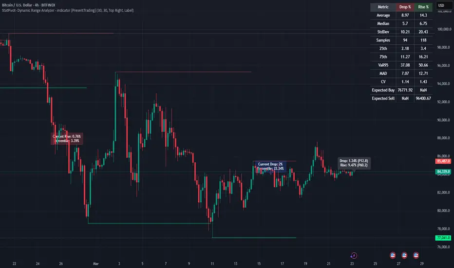
StatPivot- Dynamic Range Analyzer - indicator [PresentTrading]Hello everyone! In the following few open scripts, I would like to share various statistical tools that benefit trading. For this time, it is a powerful indicator called StatPivot- Dynamic Range Analyzer that brings a whole new dimension to your technical analysis toolkit.
This tool goes beyond traditional pivot point analysis by providing comprehensive statistical insights about price movements, helping you identify high-probability trading opportunities based on historical data patterns rather than subjective interpretations. Whether you're a day trader, swing trader, or position trader, StatPivot's real-time percentile rankings give you a statistical edge in understanding exactly where current price action stands within historical contexts.
Welcome to share your opinions! Looking forward to sharing the next tool soon!
█ Introduction and How it is Different
StatPivot is an advanced technical analysis tool that revolutionizes retracement analysis. Unlike traditional pivot indicators that only show static support/resistance levels, StatPivot delivers dynamic statistical insights based on historical pivot patterns.
Its key innovation is real-time percentile calculation - while conventional tools require new pivot formations before updating (often too late for trading decisions), StatPivot continuously analyzes where current price stands within historical retracement distributions.
Furthermore, StatPivot provides comprehensive statistical metrics including mean, median, standard deviation, and percentile distributions of price movements, giving traders a probabilistic edge by revealing which price levels represent statistically significant zones for potential reversals or continuations. By transforming raw price data into statistical insights, StatPivot helps traders move beyond subjective price analysis to evidence-based decision making.
█ Strategy, How it Works: Detailed Explanation
🔶 Pivot Point Detection and Analysis
The core of StatPivot's functionality begins with identifying significant pivot points in the price structure. Using the parameters left and right, the indicator locates pivot highs and lows by examining a specified number of bars to the left and right of each potential pivot point:
Copyp_low = ta.pivotlow(low, left, right)
p_high = ta.pivothigh(high, left, right)
For a point to qualify as a pivot low, it must have left higher lows to its left and right higher lows to its right. Similarly, a pivot high must have left lower highs to its left and right lower highs to its right. This approach ensures that only significant turning points are recognized.
🔶 Percentage Change Calculation
Once pivot points are identified, StatPivot calculates the percentage changes between consecutive pivot points:
For drops (when a pivot low is lower than the previous pivot low):
CopydropPercent = (previous_pivot_low - current_pivot_low) / previous_pivot_low * 100
For rises (when a pivot high is higher than the previous pivot high):
CopyrisePercent = (current_pivot_high - previous_pivot_high) / previous_pivot_high * 100
These calculations quantify the magnitude of each market swing, allowing for statistical analysis of historical price movements.
🔶 Statistical Distribution Analysis
StatPivot computes comprehensive statistics on the historical distribution of drops and rises:
Average (Mean): The arithmetic mean of all recorded percentage changes
CopyavgDrop = array.avg(dropValues)
Median: The middle value when all percentage changes are arranged in order
CopymedianDrop = array.median(dropValues)
Standard Deviation: Measures the dispersion of percentage changes from the average
CopystdDevDrop = array.stdev(dropValues)
Percentiles (25th, 75th): Values below which 25% and 75% of observations fall
Copyq1 = array.get(sorted, math.floor(cnt * 0.25))
q3 = array.get(sorted, math.floor(cnt * 0.75))
VaR95: The maximum expected percentage drop with 95% confidence
Copyvar95D = array.get(sortedD, math.floor(nD * 0.95))
Coefficient of Variation (CV): Measures relative variability
CopycvD = stdDevDrop / avgDrop
These statistics provide a comprehensive view of market behavior, enabling traders to understand the typical ranges and extreme moves.
🔶 Real-time Percentile Ranking
StatPivot's most innovative feature is its real-time percentile calculation. For each current price, it calculates:
The percentage drop from the latest pivot high:
CopycurrentDropPct = (latestPivotHigh - close) / latestPivotHigh * 100
The percentage rise from the latest pivot low:
CopycurrentRisePct = (close - latestPivotLow) / latestPivotLow * 100
The percentile ranks of these values within the historical distribution:
CopyrealtimeDropRank = (count of historical drops <= currentDropPct) / total drops * 100
This calculation reveals exactly where the current price movement stands in relation to all historical movements, providing crucial context for decision-making.
🔶 Cluster Analysis
To identify the most common retracement zones, StatPivot performs a cluster analysis by dividing the range of historical drops into five equal intervals:
CopyrangeSize = maxVal - minVal
For each interval boundary:
Copyboundaries = minVal + rangeSize * i / 5
By counting the number of observations in each interval, the indicator identifies the most frequently occurring retracement zones, which often serve as significant support or resistance areas.
🔶 Expected Price Targets
Using the statistical data, StatPivot calculates expected price targets:
CopytargetBuyPrice = close * (1 - avgDrop / 100)
targetSellPrice = close * (1 + avgRise / 100)
These targets represent statistically probable price levels for potential entries and exits based on the average historical behavior of the market.
█ Trade Direction
StatPivot functions as an analytical tool rather than a direct trading signal generator, providing statistical insights that can be applied to various trading strategies. However, the data it generates can be interpreted for different trade directions:
For Long Trades:
Entry considerations: Look for price drops that reach the 70-80th percentile range in the historical distribution, suggesting a statistically significant retracement
Target setting: Use the Expected Sell price or consider the average rise percentage as a reasonable target
Risk management: Set stop losses below recent pivot lows or at a distance related to the statistical volatility (standard deviation)
For Short Trades:
Entry considerations: Look for price rises that reach the 70-80th percentile range, indicating an unusual extension
Target setting: Use the Expected Buy price or average drop percentage as a target
Risk management: Set stop losses above recent pivot highs or based on statistical measures of volatility
For Range Trading:
Use the most common drop and rise clusters to identify probable reversal zones
Trade bounces between these statistically significant levels
For Trend Following:
Confirm trend strength by analyzing consecutive higher pivot lows (uptrend) or lower pivot highs (downtrend)
Use lower percentile retracements (20-30th percentile) as entry opportunities in established trends
█ Usage
StatPivot offers multiple ways to integrate its statistical insights into your trading workflow:
Statistical Table Analysis: Review the comprehensive statistics displayed in the data table to understand the market's behavior. Pay particular attention to:
Average drop and rise percentages to set reasonable expectations
Standard deviation to gauge volatility
VaR95 for risk assessment
Real-time Percentile Monitoring: Watch the real-time percentile display to see where the current price movement stands within the historical distribution. This can help identify:
Extreme movements (90th+ percentile) that might indicate reversal opportunities
Typical retracements (40-60th percentile) that might continue further
Shallow pullbacks (10-30th percentile) that might represent continuation opportunities in trends
Support and Resistance Identification: Utilize the plotted pivot points as key support and resistance levels, especially when they align with statistically significant percentile ranges.
Target Price Setting: Use the expected buy and sell prices calculated from historical averages as initial targets for your trades.
Risk Management: Apply the statistical measurements like standard deviation and VaR95 to set appropriate stop loss levels that account for the market's historical volatility.
Pattern Recognition: Over time, learn to recognize when certain percentile levels consistently lead to reversals or continuations in your specific market, and develop personalized strategies based on these observations.
█ Default Settings
The default settings of StatPivot have been carefully calibrated to provide reliable statistical analysis across a variety of markets and timeframes, but understanding their effects allows for optimal customization:
Left Bars (30) and Right Bars (30): These parameters determine how pivot points are identified. With both set to 30 by default:
A pivot low must be the lowest point among 30 bars to its left and 30 bars to its right
A pivot high must be the highest point among 30 bars to its left and 30 bars to its right
Effect on performance: Larger values create fewer but more significant pivot points, reducing noise but potentially missing important market structures. Smaller values generate more pivot points, capturing more nuanced movements but potentially including noise.
Table Position (Top Right): Determines where the statistical data table appears on the chart.
Effect on performance: No impact on analytical performance, purely a visual preference.
Show Distribution Histogram (False): Controls whether the distribution histogram of drop percentages is displayed.
Effect on performance: Enabling this provides visual insight into the distribution of retracements but can clutter the chart.
Show Real-time Percentile (True): Toggles the display of real-time percentile rankings.
Effect on performance: A critical setting that enables the dynamic analysis of current price movements. Disabling this removes one of the key advantages of the indicator.
Real-time Percentile Display Mode (Label): Chooses between label display or indicator line for percentile rankings.
Effect on performance: Labels provide precise information at the current price point, while indicator lines show the evolution of percentile rankings over time.
Advanced Considerations for Settings Optimization:
Timeframe Adjustment: Higher timeframes generally benefit from larger Left/Right values to identify truly significant pivots, while lower timeframes may require smaller values to capture shorter-term swings.
Volatility-Based Tuning: In highly volatile markets, consider increasing the Left/Right values to filter out noise. In less volatile conditions, lower values can help identify more potential entry and exit points.
Market-Specific Optimization: Different markets (forex, stocks, commodities) display different retracement patterns. Monitor the statistics table to see if your market typically shows larger or smaller retracements than the current settings are optimized for.
Trading Style Alignment: Adjust the settings to match your trading timeframe. Day traders might prefer settings that identify shorter-term pivots (smaller Left/Right values), while swing traders benefit from more significant pivots (larger Left/Right values).
By understanding how these settings affect the analysis and customizing them to your specific market and trading style, you can maximize the effectiveness of StatPivot as a powerful statistical tool for identifying high-probability trading opportunities.
ADX Trend Strength Analyzer█ OVERVIEW
This script implements the Average Directional Index (ADX), a powerful tool used to measure the strength of market trends. It works alongside the Directional Movement Index (DMI), which breaks down the directional market pressure into bullish (+DI) and bearish (-DI) components. The purpose of the ADX is to indicate when the market is in a strong trend, without specifying the direction. This indicator can be especially useful for identifying market trends early and validating trading strategies based on trend-following systems.
The ADX component in this script is based on two key parameters:
ADX Smoothing Length (adxlen), which determines the degree of smoothing for the trend strength.
DI Length (dilen), which defines the look-back period for calculating the directional index values.
Additionally, a horizontal line is plotted at the 30 level, providing a widely used threshold that signifies when a trend is considered strong (above 30).
█ CONCEPTS
Directional Movement (DM): The core idea behind this indicator is the calculation of price movement in terms of bullish and bearish forces. By evaluating the change in highs and lows, the script distinguishes between bullish movement (+DM) and bearish movement (-DM). These values are normalized by dividing them by the True Range (TR), creating the +DI and -DI values.
True Range (TR): The True Range is calculated using the Average True Range (ATR) formula, and it serves to smooth out volatility, ensuring that short-term fluctuations don't distort the long-term trend signal.
ADX Calculation: The ADX is derived from the absolute difference between the +DI and -DI. By smoothing this difference and normalizing it, the ADX is able to measure the overall strength of the trend without regard to whether the market is moving up or down. A rising ADX indicates increasing trend strength, while a falling ADX signals weakening trends.
█ METHODOLOGY
Directional Movement Calculation: The script first determines the upward and downward price movement by comparing changes in the high and low prices. If the upward movement is greater than the downward movement, it registers a bullish signal and vice versa for bearish movement.
True Range Adjustment: The script then applies a smoothing function to normalize these movements by dividing them by the True Range (ATR). This ensures that the trend signal is based on relative, rather than absolute, price movements.
ADX Signal Generation: The final step is to calculate the ADX by applying the Relative Moving Average (RMA) to the difference between +DI and -DI. This produces the ADX value, which is plotted in red, making it easy to visualize shifts in market momentum.
Threshold Line: A blue horizontal line is plotted at 30, which serves as a key reference point. When the ADX is above this line, it indicates a strong trend, whether bullish or bearish.
█ HOW TO USE
Trend Strength: Traders typically use the 30 level as a critical threshold. When the ADX is above 30, it signifies a strong trend, making it a favorable environment for trend-following strategies. Conversely, ADX values below 30 suggest a weak or non-trending market.
+DI and -DI Relationship: The indicator also provides insight into whether the trend is bullish or bearish. When +DI is greater than -DI, the market is considered bullish. When -DI is greater than +DI, the market is considered bearish. While this script focuses on the ADX value itself, the underlying +DI and -DI help interpret the trend direction.
Market Conditions: This indicator is effective in trending markets, but not ideal for choppy or sideways conditions. Traders can use it to determine the best entry and exit points when trends are strong, or to avoid trading in periods of low volatility.
Combining with Other Indicators: The ADX is commonly used in conjunction with oscillators like RSI or moving averages, to confirm the trend strength and avoid false signals.
█ METHOD VARIANTS
This script applies the standard approach for calculating the ADX, but could be adapted with the following variants:
Different Timeframes: The script could be modified to calculate ADX values across higher or lower timeframes, depending on the trader's strategy.
Custom Thresholds: Instead of using the default 30 threshold, traders could adjust the horizontal line to suit their own risk tolerance or market conditions.

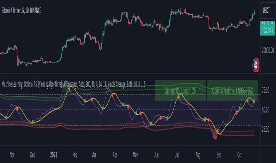
Machine Learning: Optimal RSI [YinYangAlgorithms]This Indicator, will rate multiple different lengths of RSIs to determine which RSI to RSI MA cross produced the highest profit within the lookback span. This ‘Optimal RSI’ is then passed back, and if toggled will then be thrown into a Machine Learning calculation. You have the option to Filter RSI and RSI MA’s within the Machine Learning calculation. What this does is, only other Optimal RSI’s which are in the same bullish or bearish direction (is the RSI above or below the RSI MA) will be added to the calculation.
You can either (by default) use a Simple Average; which is essentially just a Mean of all the Optimal RSI’s with a length of Machine Learning. Or, you can opt to use a k-Nearest Neighbour (KNN) calculation which takes a Fast and Slow Speed. We essentially turn the Optimal RSI into a MA with different lengths and then compare the distance between the two within our KNN Function.
RSI may very well be one of the most used Indicators for identifying crucial Overbought and Oversold locations. Not only that but when it crosses its Moving Average (MA) line it may also indicate good locations to Buy and Sell. Many traders simply use the RSI with the standard length (14), however, does that mean this is the best length?
By using the length of the top performing RSI and then applying some Machine Learning logic to it, we hope to create what may be a more accurate, smooth, optimal, RSI.
Tutorial:
This is a pretty zoomed out Perspective of what the Indicator looks like with its default settings (except with Bollinger Bands and Signals disabled). If you look at the Tables above, you’ll notice, currently the Top Performing RSI Length is 13 with an Optimal Profit % of: 1.00054973. On its default settings, what it does is Scan X amount of RSI Lengths and checks for when the RSI and RSI MA cross each other. It then records the profitability of each cross to identify which length produced the overall highest crossing profitability. Whichever length produces the highest profit is then the RSI length that is used in the plots, until another length takes its place. This may result in what we deem to be the ‘Optimal RSI’ as it is an adaptive RSI which changes based on performance.
In our next example, we changed the ‘Optimal RSI Type’ from ‘All Crossings’ to ‘Extremity Crossings’. If you compare the last two examples to each other, you’ll notice some similarities, but overall they’re quite different. The reason why is, the Optimal RSI is calculated differently. When using ‘All Crossings’ everytime the RSI and RSI MA cross, we evaluate it for profit (short and long). However, with ‘Extremity Crossings’, we only evaluate it when the RSI crosses over the RSI MA and RSI <= 40 or RSI crosses under the RSI MA and RSI >= 60. We conclude the crossing when it crosses back on its opposite of the extremity, and that is how it finds its Optimal RSI.
The way we determine the Optimal RSI is crucial to calculating which length is currently optimal.
In this next example we have zoomed in a bit, and have the full default settings on. Now we have signals (which you can set alerts for), for when the RSI and RSI MA cross (green is bullish and red is bearish). We also have our Optimal RSI Bollinger Bands enabled here too. These bands allow you to see where there may be Support and Resistance within the RSI at levels that aren’t static; such as 30 and 70. The length the RSI Bollinger Bands use is the Optimal RSI Length, allowing it to likewise change in correlation to the Optimal RSI.
In the example above, we’ve zoomed out as far as the Optimal RSI Bollinger Bands go. You’ll notice, the Bollinger Bands may act as Support and Resistance locations within and outside of the RSI Mid zone (30-70). In the next example we will highlight these areas so they may be easier to see.
Circled above, you may see how many times the Optimal RSI faced Support and Resistance locations on the Bollinger Bands. These Bollinger Bands may give a second location for Support and Resistance. The key Support and Resistance may still be the 30/50/70, however the Bollinger Bands allows us to have a more adaptive, moving form of Support and Resistance. This helps to show where it may ‘bounce’ if it surpasses any of the static levels (30/50/70).
Due to the fact that this Indicator may take a long time to execute and it can throw errors for such, we have added a Setting called: Adjust Optimal RSI Lookback and RSI Count. This settings will automatically modify the Optimal RSI Lookback Length and the RSI Count based on the Time Frame you are on and the Bar Indexes that are within. For instance, if we switch to the 1 Hour Time Frame, it will adjust the length from 200->90 and RSI Count from 30->20. If this wasn’t adjusted, the Indicator would Timeout.
You may however, change the Setting ‘Adjust Optimal RSI Lookback and RSI Count’ to ‘Manual’ from ‘Auto’. This will give you control over the ‘Optimal RSI Lookback Length’ and ‘RSI Count’ within the Settings. Please note, it will likely take some “fine tuning” to find working settings without the Indicator timing out, but there are definitely times you can find better settings than our ‘Auto’ will create; especially on higher Time Frames. The Minimum our ‘Auto’ will create is:
Optimal RSI Lookback Length: 90
RSI Count: 20
The Maximum it will create is:
Optimal RSI Lookback Length: 200
RSI Count: 30
If there isn’t much bar index history, for instance, if you’re on the 1 Day and the pair is BTC/USDT you’ll get < 4000 Bar Indexes worth of data. For this reason it is possible to manually increase the settings to say:
Optimal RSI Lookback Length: 500
RSI Count: 50
But, please note, if you make it too high, it may also lead to inaccuracies.
We will conclude our Tutorial here, hopefully this has given you some insight as to how calculating our Optimal RSI and then using it within Machine Learning may create a more adaptive RSI.
Settings:
Optimal RSI:
Show Crossing Signals: Display signals where the RSI and RSI Cross.
Show Tables: Display Information Tables to show information like, Optimal RSI Length, Best Profit, New Optimal RSI Lookback Length and New RSI Count.
Show Bollinger Bands: Show RSI Bollinger Bands. These bands work like the TDI Indicator, except its length changes as it uses the current RSI Optimal Length.
Optimal RSI Type: This is how we calculate our Optimal RSI. Do we use all RSI and RSI MA Crossings or just when it crosses within the Extremities.
Adjust Optimal RSI Lookback and RSI Count: Auto means the script will automatically adjust the Optimal RSI Lookback Length and RSI Count based on the current Time Frame and Bar Index's on chart. This will attempt to stop the script from 'Taking too long to Execute'. Manual means you have full control of the Optimal RSI Lookback Length and RSI Count.
Optimal RSI Lookback Length: How far back are we looking to see which RSI length is optimal? Please note the more bars the lower this needs to be. For instance with BTC/USDT you can use 500 here on 1D but only 200 for 15 Minutes; otherwise it will timeout.
RSI Count: How many lengths are we checking? For instance, if our 'RSI Minimum Length' is 4 and this is 30, the valid RSI lengths we check is 4-34.
RSI Minimum Length: What is the RSI length we start our scans at? We are capped with RSI Count otherwise it will cause the Indicator to timeout, so we don't want to waste any processing power on irrelevant lengths.
RSI MA Length: What length are we using to calculate the optimal RSI cross' and likewise plot our RSI MA with?
Extremity Crossings RSI Backup Length: When there is no Optimal RSI (if using Extremity Crossings), which RSI should we use instead?
Machine Learning:
Use Rational Quadratics: Rationalizing our Close may be beneficial for usage within ML calculations.
Filter RSI and RSI MA: Should we filter the RSI's before usage in ML calculations? Essentially should we only use RSI data that are of the same type as our Optimal RSI? For instance if our Optimal RSI is Bullish (RSI > RSI MA), should we only use ML RSI's that are likewise bullish?
Machine Learning Type: Are we using a Simple ML Average, KNN Mean Average, KNN Exponential Average or None?
KNN Distance Type: We need to check if distance is within the KNN Min/Max distance, which distance checks are we using.
Machine Learning Length: How far back is our Machine Learning going to keep data for.
k-Nearest Neighbour (KNN) Length: How many k-Nearest Neighbours will we account for?
Fast ML Data Length: What is our Fast ML Length? This is used with our Slow Length to create our KNN Distance.
Slow ML Data Length: What is our Slow ML Length? This is used with our Fast Length to create our KNN Distance.
If you have any questions, comments, ideas or concerns please don't hesitate to contact us.
HAPPY TRADING!
vol_rangesThis script shows three measures of volatility:
historical (hv): realized volatility of the recent past
median (mv): a long run average of realized volatility
implied (iv): a user-defined volatility
Historical and median volatility are based on the EWMA, rather than standard deviation, method of calculating volatility. Since Tradingview's built in ema function uses a window, the "window" parameter determines how much historical data is used to calculate these volatility measures. E.g. 30 on a daily chart means the previous 30 days.
The plots above and below historical candles show past projections based on these measures. The "periods to expiration" dictates how far the projection extends. At 30 periods to expiration (default), the plot will indicate the one standard deviation range from 30 periods ago. This is calculated by multiplying the volatility measure by the square root of time. For example, if the historical volatility (hv) was 20% and the window is 30, then the plot is drawn over: close * 1.2 * sqrt(30/252).
At the most recent candle, this same calculation is simply drawn as a line projecting into the future.
This script is intended to be used with a particular options contract in mind. For example, if the option expires in 15 days and has an implied volatility of 25%, choose 15 for the window and 25 for the implied volatility options. The ranges drawn will reflect the two standard deviation range both in the future (lines) and at any point in the past (plots) for HV (blue), MV (red), and IV (grey).

Volume Profile [Makit0]VOLUME PROFILE INDICATOR v0.5 beta
Volume Profile is suitable for day and swing trading on stock and futures markets, is a volume based indicator that gives you 6 key values for each session: POC, VAH, VAL, profile HIGH, LOW and MID levels. This project was born on the idea of plotting the RTH sessions Value Areas for /ES in an automated way, but you can select between 3 different sessions: RTH, GLOBEX and FULL sessions.
Some basic concepts:
- Volume Profile calculates the total volume for the session at each price level and give us market generated information about what price and range of prices are the most traded (where the value is)
- Value Area (VA): range of prices where 70% of the session volume is traded
- Value Area High (VAH): highest price within VA
- Value Area Low (VAL): lowest price within VA
- Point of Control (POC): the most traded price of the session (with the most volume)
- Session HIGH, LOW and MID levels are also important
There are a huge amount of things to know of Market Profile and Auction Theory like types of days, types of openings, relationships between value areas and openings... for those interested Jim Dalton's work is the way to come
I'm in my 2nd trading year and my goal for this year is learning to daytrade the futures markets thru the lens of Market Profile
For info on Volume Profile: TV Volume Profile wiki page at www.tradingview.com
For info on Market Profile and Market Auction Theory: Jim Dalton's book Mind over markets (this is a MUST)
BE AWARE: this indicator is based on the current chart's time interval and it only plots on 1, 2, 3, 5, 10, 15 and 30 minutes charts.
This is the correlation table TV uses in the Volume Profile Session Volume indicator (from the wiki above)
Chart Indicator
1 - 5 1
6 - 15 5
16 - 30 10
31 - 60 15
61 - 120 30
121 - 1D 60
This indicator doesn't follow that correlation, it doesn't get the volume data from a lower timeframe, it gets the data from the current chart resolution.
FEATURES
- 6 key values for each session: POC (solid yellow), VAH (solid red), VAL (solid green), profile HIGH (dashed silver), LOW (dashed silver) and MID (dotted silver) levels
- 3 sessions to choose for: RTH, GLOBEX and FULL
- select the numbers of sessions to plot by adding 12 hours periods back in time
- show/hide POC
- show/hide VAH & VAL
- show/hide session HIGH, LOW & MID levels
- highlight the periods of time out of the session (silver)
- extend the plotted lines all the way to the right, be careful this can turn the chart unreadable if there are a lot of sessions and lines plotted
SETTINGS
- Session: select between RTH (8:30 to 15:15 CT), GLOBEX (17:00 to 8:30 CT) and FULL (17:00 to 15:15 CT) sessions. RTH by default
- Last 12 hour periods to show: select the deph of the study by adding periods, for example, 60 periods are 30 natural days and around 22 trading days. 1 period by default
- Show POC (Point of Control): show/hide POC line. true by default
- Show VA (Value Area High & Low): show/hide VAH & VAL lines. true by default
- Show Range (Session High, Low & Mid): show/hide session HIGH, LOW & MID lines. true by default
- Highlight out of session: show/hide a silver shadow over the non session periods. true by default
- Extension: Extend all the plotted lines to the right. false by default
HOW TO SETUP
BE AWARE THIS INDICATOR PLOTS ONLY IN THE FOLLOWING CHART RESOLUTIONS: 1, 2, 3, 5, 10, 15 AND 30 MINUTES CHARTS. YOU MUST SELECT ONE OF THIS RESOLUTIONS TO THE INDICATOR BE ABLE TO PLOT
- By default this indicator plots all the levels for the last RTH session within the last 12 hours, if there is no plot try to adjust the 12 hours periods until the seesion and the periods match
- For Globex/Full sessions just select what you want from the dropdown menu and adjust the periods to plot the values
- Show or hide the levels you want with the 3 groups: POC line, VA lines and Session Range lines
- The highlight and extension options are for a better visibility of the levels as POC or VAH/VAL
THANKS TO
@watsonexchange for all the help, ideas and insights on this and the last two indicators (Market Delta & Market Internals) I'm working on my way to a 'clean chart' but for me it's not an easy path
@PineCoders for all the amazing stuff they do and all the help and tools they provide, in special the Script-Stopwatch at that was key in lowering this indicator's execution time
All the TV and Pine community, open source and shared knowledge are indeed the best way to help each other
IF YOU REALLY LIKE THIS WORK, please send me a comment or a private message and TELL ME WHAT you trade, HOW you trade it and your FAVOURITE SETUP for pulling out money from the market in a consistent basis, I'm learning to trade (this is my 2nd year) and I need all the help I can get
GOOD LUCK AND HAPPY TRADING

Sav Fx Dynamic P & D°//@version=5
indicator("Sav Fx Dynamic P & D°", overlay = true, max_boxes_count = 50, max_labels_count = 2, max_lines_count = 10)
// Global Settings (visible)
customLineColor = input.color(#000000, "True Open", group = "Global Settings")
// Input for custom sessionTypeText size and width
sessionTypeTextSize = input.string("small", "Session Type Text Size", options= , group="Text Settings")
// On/Off switches for each open line
show90MinuteCycleOpen = input.bool(true, "90 Minute Cycle Open", group="Open Lines")
showTrueNewYorkOpen = input.bool(true, "True New York Open", group="Open Lines")
showTrueDayOpen = input.bool(true, "True Day Open", group="Open Lines")
showTrueWeekOpen = input.bool(true, "True Week Open", group="Open Lines")
showTrueMonthOpen = input.bool(false, "True Month Open", group="Open Lines")
IsTime(h, m, timezone) =>
not na(time) and hour(time, timezone) == h and minute(time, timezone) == m
IsSession(sess, timezone) =>
not na(time(timeframe.period, sess, timezone))
is6_00Session = IsSession("0600-0730", "America/New_York")
is7_30Session = IsSession("0730-0900", "America/New_York")
is9_00Session = IsSession("0900-1030", "America/New_York")
is10_30Session = IsSession("1030-1200", "America/New_York")
var MOPLine = line.new(na, na, na, na, color = customLineColor, width = 1, style = line.style_dashed)
var MOPLabel = label.new(na, na, text = "True Day Open", color = color.rgb(120, 123, 134, 100), textcolor = customLineColor, size = size.small, style = label.style_label_left)
var float trueDayOpen = na
if showTrueDayOpen
if IsTime(0, 0, "America/New_York")
line.set_xy1(MOPLine, bar_index, open)
line.set_xy2(MOPLine, bar_index, open)
label.set_xy(MOPLabel, bar_index, open)
trueDayOpen := open
if barstate.islast
line.set_x2(MOPLine, bar_index + 20)
label.set_x(MOPLabel, bar_index + 20)
else
line.delete(MOPLine)
label.delete(MOPLabel)
var NYTrueOpenLine = line.new(na, na, na, na, color = customLineColor, width = 1, style = line.style_dashed)
var NYTrueOpenLabel = label.new(na, na, text = "True New York Open", color = color.rgb(105, 130, 218, 100), textcolor = customLineColor, size = size.small, style = label.style_label_left)
var float NYTrueOpen = na
if showTrueNewYorkOpen
if IsTime(1, 30, "America/New_York") or IsTime(7, 30, "America/New_York") or IsTime(13, 30, "America/New_York")
line.set_xy1(NYTrueOpenLine, bar_index, open)
line.set_xy2(NYTrueOpenLine, bar_index, open)
label.set_xy(NYTrueOpenLabel, bar_index, open)
NYTrueOpen := open
if IsTime(1, 30, "America/New_York")
label.set_text(NYTrueOpenLabel, "True London Open")
if IsTime(7, 30, "America/New_York")
label.set_text(NYTrueOpenLabel, "True New York Open")
if IsTime(13, 30, "America/New_York")
label.set_text(NYTrueOpenLabel, "True PM Session Open")
if barstate.islast
line.set_x2(NYTrueOpenLine, bar_index + 20)
label.set_x(NYTrueOpenLabel, bar_index + 20)
else
line.delete(NYTrueOpenLine)
label.delete(NYTrueOpenLabel)
var lookahead_bars = 20
var MondayLine = line.new(na, na, na, na, color = customLineColor, width = 1, style = line.style_dashed)
var MondayLabel = label.new(na, na, text = timeframe.isintraday and timeframe.multiplier >= 5 ? "True week Open" : "", color = #9b27b000, textcolor = customLineColor, size = size.small, style = label.style_label_left)
if showTrueWeekOpen
if dayofweek == dayofweek.monday and IsTime(18, 0, "America/New_York")
line.set_xy1(MondayLine, bar_index, close)
line.set_xy2(MondayLine, bar_index, close)
label.set_xy(MondayLabel, bar_index, close)
if barstate.islast
line.set_x2(MondayLine, bar_index + lookahead_bars)
label.set_x(MondayLabel, bar_index + lookahead_bars)
else
line.delete(MondayLine)
label.delete(MondayLabel)
var ninetyMinuteCycleLine = line.new(na, na, na, na, color = customLineColor, width = 1, style = line.style_dashed)
var ninetyMinuteCycleLabel = label.new(na, na, text = "90 Minute Cycle True Open", color = #4caf4f00, textcolor = customLineColor, size = size.small, style = label.style_label_left)
if show90MinuteCycleOpen
if IsTime(3, 23, "America/New_York") or IsTime(9, 23, "America/New_York") or IsTime(15, 23, "America/New_York")
line.set_xy1(ninetyMinuteCycleLine, bar_index, open)
line.set_xy2(ninetyMinuteCycleLine, bar_index, open)
label.set_xy(ninetyMinuteCycleLabel, bar_index, open)
if IsTime(3, 23, "America/New_York")
label.set_text(ninetyMinuteCycleLabel, "03:23 Cycle True Open")
if IsTime(9, 23, "America/New_York")
label.set_text(ninetyMinuteCycleLabel, "09:23 Cycle True Open")
if IsTime(15, 23, "America/New_York")
label.set_text(ninetyMinuteCycleLabel, "15:23 Cycle True Open")
if barstate.islast
line.set_x2(ninetyMinuteCycleLine, bar_index + lookahead_bars)
label.set_x(ninetyMinuteCycleLabel, bar_index + lookahead_bars)
else
line.delete(ninetyMinuteCycleLine)
label.delete(ninetyMinuteCycleLabel)
var monthOpenLine = line.new(na, na, na, na, color = customLineColor, width = 1, style = line.style_dashed)
var monthOpenLabel = label.new(na, na, text = "True Month Open", color = #ff990000, textcolor = customLineColor, size = size.small, style = label.style_label_left)
isSecondWeekSunday = dayofweek == dayofweek.sunday and (dayofmonth >= 8 and dayofmonth <= 14)
if showTrueMonthOpen
if isSecondWeekSunday and IsTime(18,0, "America/New_York")
line.set_xy1(monthOpenLine, bar_index, close)
line.set_xy2(monthOpenLine, bar_index + lookahead_bars, close)
label.set_xy(monthOpenLabel, bar_index, close)
if barstate.islast
line.set_x2(monthOpenLine, bar_index + lookahead_bars)
label.set_x(monthOpenLabel, bar_index + lookahead_bars)
else
line.delete(monthOpenLine)
label.delete(monthOpenLabel)
directionalBias = "N/A"
if is6_00Session or is7_30Session or is9_00Session or is10_30Session
directionalBias := open > NYTrueOpen ? "Bullish" : "Bearish"
var directionalBiasLabel = label.new(na, na, text = "Directional Bias: " + directionalBias, color = na, textcolor = customLineColor, size = size.normal, style = label.style_label_left)
if barstate.islast
label.set_x(directionalBiasLabel, bar_index + lookahead_bars)
label.set_text(directionalBiasLabel, "Directional Bias: " + directionalBias)
var float WeekOpen = na
if dayofweek == dayofweek.monday and IsTime(18, 0, "America/New_York")
WeekOpen := close
if showTrueWeekOpen
line.set_xy1(MondayLine, bar_index, close)
line.set_xy2(MondayLine, bar_index, close)
label.set_xy(MondayLabel, bar_index, close)
// New table for static session type display
var sessionTable = table.new(position.bottom_right, 1, 1, bgcolor = #b9b9bab8)
// Update the table.cell function call
if barstate.islast and not na(trueDayOpen) and not na(NYTrueOpen) and not na(WeekOpen)
var string sessionTypeText = syminfo.ticker + " Dead Zone"
var color sessionColor = color.rgb(126, 126, 126, 65)
// Check conditions and set session type text and color accordingly
if close < trueDayOpen and close < NYTrueOpen and close < WeekOpen
sessionTypeText := syminfo.ticker + " Week Discount"
sessionColor := #ba4b4b59
else if close > trueDayOpen and close > NYTrueOpen and close > WeekOpen
sessionTypeText := syminfo.ticker + " Week Premium"
sessionColor := #4b56ba5a
else if close < trueDayOpen and close < NYTrueOpen and close > WeekOpen
sessionTypeText := syminfo.ticker + " Day Discount & Week Dead Zone"
sessionColor := #ba4b4b59
else if close > trueDayOpen and close > NYTrueOpen and close < WeekOpen
sessionTypeText := syminfo.ticker + " Day premium & Week Dead Zone"
sessionColor := #4b56ba5a
// Using only size input for session type text
table.cell(sessionTable, 0, 0, sessionTypeText, bgcolor = sessionColor, text_color = color.black, text_size = sessionTypeTextSize)

ICT Sessions Ranges [SwissAlgo]ICT Session Ranges - ICT Liquidity Zones & Market Structure
OVERVIEW
This indicator identifies and visualizes key intraday trading sessions and liquidity zones based on Inner Circle Trader (ICT) methodology (AM, NY Lunch Raid, PM Session, London Raid). It tracks 'higher high' and 'lower low' price levels during specific time periods that may represent areas where market participants have placed orders (liquidity).
PURPOSE
The indicator helps traders observe:
Session-based price ranges during different market hours
Opening range gaps between market close and next day's open
Potential areas where liquidity may be concentrated and trigger price action
SESSIONS TRACKED
1. London Session (02:00-05:00 ET): Tracks price range during early London trading hours
2. AM Session (09:30-12:00 ET): Tracks price range during the morning New York session
3. NY Lunch Session (12:00-13:30 ET): Tracks price range during typical low-volume lunch period
4. PM Session (13:30-16:00 ET): Tracks price range during the afternoon New York session
CALCULATIONS
Session High/Low: The highest high and lowest low recorded during each active session period
Opening Range Gap: Calculated as the difference between the previous day's 16:00 close and the current day's 09:30 open
Gap Mitigation: A gap is considered mitigated when the price reaches 50% of the gap range
All times are based on America/New_York timezone (ET)
BACKGROUND INDICATORS
NY Trading Hours (09:30-16:00 ET): Optional gray background overlay
Asian Session (20:00-23:59 ET): Optional purple background overlay
VISUAL ELEMENTS
Horizontal lines mark session highs and lows
Subtle background boxes highlight each session range
Labels identify each session type
Orange shaded boxes indicate unmitigated opening range gaps
Dotted line at 50% gap level shows mitigation threshold
FEATURES
Toggle visibility for each session independently
Customizable colors for each session type
Automatic removal of mitigated gaps
All drawing objects use transparent backgrounds for chart clarity
ICT CONCEPTS
This tool relates to concepts discussed by Inner Circle Trader regarding liquidity pools, session-based analysis, and gap theory. The indicator assumes that session highs and lows may represent areas where liquidity is concentrated, and that opening range gaps may attract price until mitigated.
USAGE NOTES
Best used on intraday timeframes (1-15 minute charts)
All sessions are calculated based on actual price movement during specified time periods
Historical session data is preserved as new sessions develop
Gap detection only triggers at 09:30 ET market open
DISCLAIMER
This indicator is for educational and informational purposes only. It displays historical price levels and time-based calculations. Past performance of price levels is not indicative of future results. The identification of "liquidity zones" is a theoretical concept and does not guarantee that orders exist at these levels or that prices will react to them. Trading involves substantial risk of loss. Users should conduct their own analysis and risk assessment before making any trading decisions.
TIME ZONE
Set your timezone to: America/New_York (UTC-5)

LibTmFrLibrary "LibTmFr"
This is a utility library for handling timeframes and
multi-timeframe (MTF) analysis in Pine Script. It provides a
collection of functions designed to handle common tasks related
to period detection, session alignment, timeframe construction,
and time calculations, forming a foundation for
MTF indicators.
Key Capabilities:
1. **MTF Period Engine:** The library includes functions for
managing higher-timeframe (HTF) periods.
- **Period Detection (`isNewPeriod`):** Detects the first bar
of a given timeframe. It includes custom logic to handle
multi-month and multi-year intervals where
`timeframe.change()` may not be sufficient.
- **Bar Counting (`sinceNewPeriod`):** Counts the number of
bars that have passed in the current HTF period or
returns the final count for a completed historical period.
2. **Automatic Timeframe Selection:** Offers functions for building
a top-down analysis framework:
- **Automatic HTF (`autoHTF`):** Suggests a higher timeframe
(HTF) for broader context based on the current timeframe.
- **Automatic LTF (`autoLTF`):** Suggests an appropriate lower
timeframe (LTF) for granular intra-bar analysis.
3. **Timeframe Manipulation and Comparison:** Includes tools for
working with timeframe strings:
- **Build & Split (`buildTF`, `splitTF`):** Functions to
programmatically construct valid Pine Script timeframe
strings (e.g., "4H") and parse them back into their
numeric and unit components.
- **Comparison (`isHigherTF`, `isActiveTF`, `isLowerTF`):**
A set of functions to check if a given timeframe is
higher, lower, or the same as the script's active timeframe.
- **Multiple Validation (`isMultipleTF`):** Checks if a
higher timeframe is a practical multiple of the current
timeframe. This is based on the assumption that checking
if recent, completed HTF periods contained more than one
bar is a valid proxy for preventing data gaps.
4. **Timestamp Interpolation:** Contains an `interpTimestamp()`
function that calculates an absolute timestamp by
interpolating at a given percentage across a specified
range of bars (e.g., 50% of the way through the last
20 bars), enabling time calculations at a resolution
finer than the chart's native bars.
---
**DISCLAIMER**
This library is provided "AS IS" and for informational and
educational purposes only. It does not constitute financial,
investment, or trading advice.
The author assumes no liability for any errors, inaccuracies,
or omissions in the code. Using this library to build
trading indicators or strategies is entirely at your own risk.
As a developer using this library, you are solely responsible
for the rigorous testing, validation, and performance of any
scripts you create based on these functions. The author shall
not be held liable for any financial losses incurred directly
or indirectly from the use of this library or any scripts
derived from it.
buildTF(quantity, unit)
Builds a Pine Script timeframe string from a numeric quantity and a unit enum.
The resulting string can be used with `request.security()` or `input.timeframe`.
Parameters:
quantity (int) : series int Number to specifie how many `unit` the timeframe spans.
unit (series TFUnit) : series TFUnit The size category for the bars.
Returns: series string A Pine-style timeframe identifier, e.g.
"5S" → 5-seconds bars
"30" → 30-minute bars
"120" → 2-hour bars
"1D" → daily bars
"3M" → 3-month bars
"24M" → 2-year bars
splitTF(tf)
Splits a Pine‑timeframe identifier into numeric quantity and unit (TFUnit).
Parameters:
tf (string) : series string Timeframe string, e.g.
"5S", "30", "120", "1D", "3M", "24M".
Returns:
quantity series int The numeric value of the timeframe (e.g., 15 for "15", 3 for "3M").
unit series TFUnit The unit of the timeframe (e.g., TFUnit.minutes, TFUnit.months).
Notes on strings without a suffix:
• Pure digits are minutes; if divisible by 60, they are treated as hours.
• An "M" suffix is months; if divisible by 12, it is converted to years.
autoHTF(tf)
Picks an appropriate **higher timeframe (HTF)** relative to the selected timeframe.
It steps up along a coarse ladder to produce sensible jumps for top‑down analysis.
Mapping → chosen HTF:
≤ 1 min → 60 (1h) ≈ ×60
≤ 3 min → 180 (3h) ≈ ×60
≤ 5 min → 240 (4h) ≈ ×48
≤ 15 min → D (1 day) ≈ ×26–×32 (regular session 6.5–8 h)
> 15 min → W (1 week) ≈ ×64–×80 for 30m; varies with input
≤ 1 h → W (1 week) ≈ ×32–×40
≤ 4 h → M (1 month) ≈ ×36–×44 (~22 trading days / month)
> 4 h → 3M (3 months) ≈ ×36–×66 (e.g., 12h→×36–×44; 8h→×53–×66)
≤ 1 day → 3M (3 months) ≈ ×60–×66 (~20–22 trading days / month)
> 1 day → 12M (1 year) ≈ ×(252–264)/quantity
≤ 1 week → 12M (1 year) ≈ ×52
> 1 week → 48M (4 years) ≈ ×(208)/quantity
= 1 M → 48M (4 years) ≈ ×48
> 1 M → error ("HTF too big")
any → error ("HTF too big")
Notes:
• Inputs in months or years are restricted: only 1M is allowed; larger months/any years throw.
• Returns a Pine timeframe string usable in `request.security()` and `input.timeframe`.
Parameters:
tf (string) : series string Selected timeframe (e.g., "D", "240", or `timeframe.period`).
Returns: series string Suggested higher timeframe.
autoLTF(tf)
Selects an appropriate **lower timeframe LTF)** for intra‑bar evaluation
based on the selected timeframe. The goal is to keep intra‑bar
loops performant while providing enough granularity.
Mapping → chosen LTF:
≤ 1 min → 1S ≈ ×60
≤ 5 min → 5S ≈ ×60
≤ 15 min → 15S ≈ ×60
≤ 30 min → 30S ≈ ×60
> 30 min → 60S (1m) ≈ ×31–×59 (for 31–59 minute charts)
≤ 1 h → 1 (1m) ≈ ×60
≤ 2 h → 2 (2m) ≈ ×60
≤ 4 h → 5 (5m) ≈ ×48
> 4 h → 15 (15m) ≈ ×24–×48 (e.g., 6h→×24, 8h→×32, 12h→×48)
≤ 1 day → 15 (15m) ≈ ×26–×32 (regular sessions ~6.5–8h)
> 1 day → 60 (60m) ≈ ×(26–32) per day × quantity
≤ 1 week → 60 (60m) ≈ ×32–×40 (≈5 sessions of ~6.5–8h)
> 1 week → 240 (4h) ≈ ×(8–10) per week × quantity
≤ 1 M → 240 (4h) ≈ ×33–×44 (~20–22 sessions × 6.5–8h / 4h)
≤ 3 M → D (1d) ≈ ×(20–22) per month × quantity
> 3 M → W (1w) ≈ ×(4–5) per month × quantity
≤ 1 Y → W (1w) ≈ ×52
> 1 Y → M (1M) ≈ ×12 per year × quantity
Notes:
• Ratios for D/W/M are given as ranges because they depend on
**regular session length** (typically ~6.5–8h, not 24h).
• Returned strings can be used with `request.security()` and `input.timeframe`.
Parameters:
tf (string) : series string Selected timeframe (e.g., "D", "240", or timeframe.period).
Returns: series string Suggested lower TF to use for intra‑bar work.
isNewPeriod(tf, offset)
Returns `true` when a new session-aligned period begins, or on the Nth bar of that period.
Parameters:
tf (string) : series string Target higher timeframe (e.g., "D", "W", "M").
offset (simple int) : simple int 0 → checks for the first bar of the new period.
1+ → checks for the N-th bar of the period.
Returns: series bool `true` if the condition is met.
sinceNewPeriod(tf, offset)
Counts how many bars have passed within a higher timeframe (HTF) period.
For daily, weekly, and monthly resolutions, the period is aligned with the trading session.
Parameters:
tf (string) : series string Target parent timeframe (e.g., "60", "D").
offset (simple int) : simple int 0 → Running count for the current period.
1+ → Finalized count for the Nth most recent *completed* period.
Returns: series int Number of bars.
isHigherTF(tf, main)
Returns `true` when the selected timeframe represents a
higher resolution than the active timeframe.
Parameters:
tf (string) : series string Selected timeframe.
main (bool) : series bool When `true`, the comparison is made against the chart's main timeframe
instead of the script's active timeframe. Optional. Defaults to `false`.
Returns: series bool `true` if `tf` > active TF; otherwise `false`.
isActiveTF(tf, main)
Returns `true` when the selected timeframe represents the
exact resolution of the active timeframe.
Parameters:
tf (string) : series string Selected timeframe.
main (bool) : series bool When `true`, the comparison is made against the chart's main timeframe
instead of the script's active timeframe. Optional. Defaults to `false`.
Returns: series bool `true` if `tf` == active TF; otherwise `false`.
isLowerTF(tf, main)
Returns `true` when the selected timeframe represents a
lower resolution than the active timeframe.
Parameters:
tf (string) : series string Selected timeframe.
main (bool) : series bool When `true`, the comparison is made against the chart's main timeframe
instead of the script's active timeframe. Optional. Defaults to `false`.
Returns: series bool `true` if `tf` < active TF; otherwise `false`.
isMultipleTF(tf)
Returns `true` if the selected timeframe (`tf`) is a practical multiple
of the active skript's timeframe. It verifies this by checking if `tf` is a higher timeframe
that has consistently contained more than one bar of the skript's timeframe in recent periods.
The period detection is session-aware.
Parameters:
tf (string) : series string The higher timeframe to check.
Returns: series bool `true` if `tf` is a practical multiple; otherwise `false`.
interpTimestamp(offStart, offEnd, pct)
Calculates a precise absolute timestamp by interpolating within a bar range based on a percentage.
This version works with RELATIVE bar offsets from the current bar.
Parameters:
offStart (int) : series int The relative offset of the starting bar (e.g., 10 for 10 bars ago).
offEnd (int) : series int The relative offset of the ending bar (e.g., 1 for 1 bar ago). Must be <= offStart.
pct (float) : series float The percentage of the bar range to measure (e.g., 50.5 for 50.5%).
Values are clamped to the range.
Returns: series int The calculated, interpolated absolute Unix timestamp in milliseconds.

Luxy BIG beautiful Dynamic ORBThis is an advanced Opening Range Breakout (ORB) indicator that tracks price breakouts from the first 5, 15, 30, and 60 minutes of the trading session. It provides complete trade management including entry signals, stop-loss placement, take-profit targets, and position sizing calculations.
The ORB strategy is based on the concept that the opening range of a trading session often acts as support/resistance, and breakouts from this range tend to lead to significant moves.
What Makes This Different?
Most ORB indicators simply draw horizontal lines and leave you to figure out the rest. This indicator goes several steps further:
Multi-Stage Tracking
Instead of just one ORB timeframe, this tracks FOUR simultaneously (5min, 15min, 30min, 60min). Each stage builds on the previous one, giving you multiple trading opportunities throughout the session.
Active Trade Management
When a breakout occurs, the indicator automatically calculates and displays entry price, stop-loss, and multiple take-profit targets. These lines extend forward and update in real-time until the trade completes.
Cycle Detection
Unlike indicators that only show the first breakout, this tracks the complete cycle: Breakout → Retest → Re-breakout. You can see when price returns to test the ORB level after breaking out (potential re-entry).
Failed Breakout Warning
If price breaks out but quickly returns inside the range (within a few bars), the label changes to "FAILED BREAK" - warning you to exit or avoid the trade.
Position Sizing Calculator
Built-in risk management that tells you exactly how many shares to buy based on your account size and risk tolerance. No more guessing or manual calculations.
Advanced Filtering
Optional filters for volume confirmation, trend alignment, and Fair Value Gaps (FVG) to reduce false signals and improve win rate.
Core Features Explained
### 1. Multi-Stage ORB Levels
The indicator builds four separate Opening Range levels:
ORB 5 - First 5 minutes (fastest signals, most volatile)
ORB 15 - First 15 minutes (balanced, most popular)
ORB 30 - First 30 minutes (slower, more reliable)
ORB 60 - First 60 minutes (slowest, most confirmed)
Each level is drawn as a horizontal range on your chart. As time progresses, the ranges expand to include more price action. You can enable or disable any stage and assign custom colors to each.
How it works: During the opening minutes, the indicator tracks the highest high and lowest low. Once the time period completes, those levels become your ORB high and low for that stage.
### 2. Breakout Detection
When price closes outside the ORB range, a label appears:
BREAK UP (green label above price) - Price closed above ORB High
BREAK DOWN (red label below price) - Price closed below ORB Low
The label shows which ORB stage triggered (ORB5, ORB15, etc.) and the cycle number if tracking multiple breakouts.
Important: Signals appear on bar close only - no repainting. What you see is what you get.
### 3. Retest Detection
After price breaks out and moves away, if it returns to test the ORB level, a "RETEST" label appears (orange). This indicates:
The original breakout level is now acting as support/resistance
Potential re-entry opportunity if you missed the first breakout
Confirmation that the level is significant
The indicator requires price to move a minimum distance away before considering it a valid retest (configurable in settings).
### 4. Failed Breakout Detection
If price breaks out but returns inside the ORB range within a few bars (before the breakout is "committed"), the original label changes to "FAILED BREAK" in orange.
This warns you:
The breakout lacked conviction
Consider exiting if already in the trade
Wait for better setup
Committed Breakout: The indicator tracks how many bars price stays outside the range. Only after staying outside for the minimum number of bars does it become a committed breakout that can be retested.
### 5. TP/SL Lines (Trade Management)
When a breakout occurs, colored horizontal lines appear showing:
Entry Line (cyan for long, orange for short) - Your entry price (the ORB level)
Stop Loss Line (red) - Where to exit if trade goes against you
TP1, TP2, TP3 Lines (same color as entry) - Profit targets at 1R, 2R, 3R
These lines extend forward as new bars form, making it easy to track your trade. When a target is hit, the line turns green and the label shows a checkmark.
Lines freeze (stop updating) when:
Stop loss is hit
The final enabled take-profit is hit
End of trading session (optional setting)
### 6. Position Sizing Dashboard
The dashboard (bottom-left corner by default) shows real-time information:
Current ORB stage and range size
Breakout status (Inside Range / Break Up / Break Down)
Volume confirmation (if filter enabled)
Trend alignment (if filter enabled)
Entry and Stop Loss prices
All enabled Take Profit levels with percentages
Risk/Reward ratio
Position sizing: Max shares to buy and total risk amount
Position Sizing Example:
If your account is $25,000 and you risk 1% per trade ($250), and the distance from entry to stop loss is $0.50, the calculator shows you can buy 500 shares (250 / 0.50 = 500).
### 7. FVG Filter (Fair Value Gap)
Fair Value Gaps are price inefficiencies - gaps left by strong momentum where one candle's high doesn't overlap with a previous candle's low (or vice versa).
When enabled, this filter:
Detects bullish and bearish FVGs
Draws semi-transparent boxes around these gaps
Only allows breakout signals if there's an FVG near the breakout level
Why this helps: FVGs indicate institutional activity. Breakouts through FVGs tend to be stronger and more reliable.
Proximity setting: Controls how close the FVG must be to the ORB level. 2.0x means the breakout can be within 2 times the FVG size - a reasonable default.
### 8. Volume & Trend Filters
Volume Filter:
Requires current volume to be above average (customizable multiplier). High volume breakouts are more likely to sustain.
Set minimum multiplier (e.g., 1.5x = 50% above average)
Set "strong volume" multiplier (e.g., 2.5x) that bypasses other filters
Dashboard shows current volume ratio
Trend Filter:
Only shows breakouts aligned with a higher timeframe trend. Choose from:
VWAP - Price above/below volume-weighted average
EMA - Price above/below exponential moving average
SuperTrend - ATR-based trend indicator
Combined modes (VWAP+EMA, VWAP+SuperTrend) for stricter filtering
### 9. Pullback Filter (Advanced)
Purpose:
Waits for price to pull back slightly after initial breakout before confirming the signal.
This reduces false breakouts from immediate reversals.
How it works:
- After breakout is detected, indicator waits for a small pullback (default 2%)
- Once pullback occurs AND price breaks out again, signal is confirmed
- If no pullback within timeout period (5 bars), signal is issued anyway
Settings:
Enable Pullback Filter: Turn this filter on/off
Pullback %: How much price must pull back (2% is balanced)
Timeout (bars): Max bars to wait for pullback (5 is standard)
When to use:
- Choppy markets with many fake breakouts
- When you want higher quality signals
- Combine with Volume filter for maximum confirmation
Trade-off:
- Better signal quality
- May miss some valid fast moves
- Slight entry delay
How to Use This Indicator
### For Beginners - Simple Setup
Add the indicator to your chart (5-minute or 15-minute timeframe recommended)
Leave all default settings - they work well for most stocks
Watch for BREAK UP or BREAK DOWN labels to appear
Check the dashboard for entry, stop loss, and targets
Use the position sizing to determine how many shares to buy
Basic Trading Plan:
Wait for a clear breakout label
Enter at the ORB level (or next candle open if you're late)
Place stop loss where the red line indicates
Take profit at TP1 (50% of position) and TP2 (remaining 50%)
### For Advanced Traders - Customized Setup
Choose which ORB stages to track (you might only want ORB15 and ORB30)
Enable filters: Volume (stocks) or Trend (trending markets)
Enable FVG filter for institutional confirmation
Set "Track Cycles" mode to catch retests and re-breakouts
Customize stop loss method (ATR for volatile stocks, ORB% for stable ones)
Adjust risk per trade and account size for accurate position sizing
Advanced Strategy Example:
Enable ORB15 only (disable others for cleaner chart)
Turn on Volume filter at 1.5x with Strong at 2.5x
Enable Trend filter using VWAP
Set Signal Mode to "Track Cycles" with Max 3 cycles
Wait for aligned breakouts (Volume + Trend + Direction)
Enter on retest if you missed the initial break
### Timeframe Recommendations
5-minute chart: Scalping, very active trading, crypto
15-minute chart: Day trading, balanced approach (most popular)
30-minute chart: Swing entries, less screen time
60-minute chart: Position trading, longer holds
The indicator works on any intraday timeframe, but ORB is fundamentally a day trading strategy. Daily charts don't make sense for ORB.
DEFAULT CONFIGURATION
ON by Default:
• All 4 ORB stages (5/15/30/60)
• Breakout Detection
• Retest Labels
• All TP levels (1/1.5/2/3)
• TP/SL Lines (Detailed mode)
• Dashboard (Bottom Left, Dark theme)
• Position Size Calculator
OFF by Default (Optional Filters):
• FVG Filter
• Pullback Filter
• Volume Filter
• Trend Filter
• HTF Bias Check
• Alerts
Recommended for Beginners:
• Leave all defaults
• Session Mode: Auto-Detect
• Signal Mode: Track Cycles
• Stop Method: ATR
• Add Volume Filter if trading stocks
Recommended for Advanced:
• Enable ORB15 + ORB30 only (disable 5 & 60)
• Enable: Volume + Trend + FVG
• Signal Mode: Track Cycles, Max 3
• Stop Method: ATR or Safer
• Enable HTF Daily bias check
## Settings Guide
The settings are organized into logical groups. Here's what each section controls:
### ORB COLORS Section
Show Edge Labels: Display "ORB 5", "ORB 15" labels at the right edge of the levels
Background: Fill the area between ORB high/low with color
Transparency: How see-through the background is (95% is nearly invisible)
Enable ORB 5/15/30/60: Turn each stage on or off individually
Colors: Assign colors to each ORB stage for easy identification
### SESSION SETTINGS Section
Session Mode: Choose trading session (Auto-Detect works for most instruments)
Custom Session Hours: Define your own hours if needed (format: HHMM-HHMM)
Auto-Detect uses the instrument's natural hours (stocks use exchange hours, crypto uses 24/7).
### BREAKOUT DETECTION Section
Enable Breakout Detection: Master switch for signals
Show Retest Labels: Display retest signals
Label Size: Visual size for all labels (Small recommended)
Enable FVG Filter: Require Fair Value Gap confirmation
Show FVG Boxes: Display the gap boxes on chart
Signal Mode: "First Only" = one signal per direction per day, "Track Cycles" = multiple signals
Max Cycles: How many breakout-retest cycles to track (6 is balanced)
Breakout Buffer: Extra distance required beyond ORB level (0.1-0.2% recommended)
Min Distance for Retest: How far price must move away before retest is valid (2% recommended)
Min Bars Outside ORB: Bars price must stay outside for committed breakout (2 is balanced)
### TARGETS & RISK Section
Enable Targets & Stop-Loss: Calculate and show trade management
TP1/TP2/TP3 checkboxes: Select which profit targets to display
Stop Method: How to calculate stop loss placement
- ATR: Based on volatility (best for most cases)
- ORB %: Fixed % of ORB range
- Swing: Recent swing high/low
- Safer: Widest of all methods
ATR Length & Multiplier: Controls ATR stop distance (14 period, 1.5x is standard)
ORB Stop %: Percentage beyond ORB for stop (20% is balanced)
Swing Bars: Lookback period for swing high/low (3 is recent)
### TP/SL LINES Section
Show TP/SL Lines: Display horizontal lines on chart
Label Format: "Short" = minimal text, "Detailed" = shows prices
Freeze Lines at EOD: Stop extending lines at session close
### DASHBOARD Section
Show Info Panel: Display the metrics dashboard
Theme: Dark or Light colors
Position: Where to place dashboard on chart
Toggle rows: Show/hide specific information rows
Calculate Position Size: Enable the position sizing calculator
Risk Mode: Risk fixed $ amount or % of account
Account Size: Your total trading capital
Risk %: Percentage to risk per trade (0.5-1% recommended)
### VOLUME FILTER Section
Enable Volume Filter: Require volume confirmation
MA Length: Average period (20 is standard)
Min Volume: Required multiplier (1.5x = 50% above average)
Strong Volume: Multiplier that bypasses other filters (2.5x)
### TREND FILTER Section
Enable Trend Filter: Require trend alignment
Trend Mode: Method to determine trend (VWAP is simple and effective)
Custom EMA Length: If using EMA mode (50 for swing, 20 for day trading)
SuperTrend settings: Period and Multiplier if using SuperTrend mode
### HIGHER TIMEFRAME Section
Check Daily Trend: Display higher timeframe bias in dashboard
Timeframe: What TF to check (D = daily, recommended)
Method: Price vs MA (stable) or Candle Direction (reactive)
MA Period: EMA length for Price vs MA method (20 is balanced)
Min Strength %: Minimum strength threshold for HTF bias to be considered
- For "Price vs MA": Minimum distance (%) from moving average
- For "Candle Direction": Minimum candle body size (%)
- 0.5% is balanced - increase for stricter filtering
- Lower values = more signals, higher values = only strong trends
### ALERTS Section
Enable Alerts: Master switch (must be ON to use any alerts)
Breakout Alerts: Notify on ORB breakouts
Retest Alerts: Notify when price retests after breakout
Failed Break Alerts: Notify on failed breakouts
Stage Complete Alerts: Notify when each ORB stage finishes forming
After enabling desired alert types, click "Create Alert" button, select this indicator, choose "Any alert() function call".
## Tips & Best Practices
### General Trading Tips
ORB works best on liquid instruments (stocks with good volume, major crypto pairs)
First hour of the session is most important - that's when ORB is forming
Breakouts WITH the trend have higher success rates - use the trend filter
Failed breakouts are common - use the "Min Bars Outside" setting to filter weak moves
Not every day produces good ORB setups - be patient and selective
### Position Sizing Best Practices
Never risk more than 1-2% of your account on a single trade
Use the built-in calculator - don't guess your position size
Update your account size monthly as it grows
Smaller accounts: use $ Amount mode for simplicity
Larger accounts: use % of Account mode for scaling
### Take Profit Strategy
Most traders use: 50% at TP1, 50% at TP2
Aggressive: Hold through TP1 for TP2 or TP3
Conservative: Full exit at TP1 (1:1 risk/reward)
After TP1 hits, consider moving stop to breakeven
TP3 rarely hits - only on strong trending days
### Filter Combinations
Maximum Quality: Volume + Trend + FVG (fewest signals, highest quality)
Balanced: Volume + Trend (good quality, reasonable frequency)
Active Trading: No filters or Volume only (many signals, lower quality)
Trending Markets: Trend filter essential (indices, crypto)
Range-Bound: Volume + FVG (avoid trend filter)
### Common Mistakes to Avoid
Chasing breakouts - wait for the bar to close, don't FOMO into wicks
Ignoring the stop loss - always use it, move it manually if needed
Over-leveraging - the calculator shows MAX shares, you can buy less
Trading every signal - quality > quantity, use filters
Not tracking results - keep a journal to see what works for YOU
## Pros and Cons
### Advantages
Complete all-in-one solution - from signal to position sizing
Multiple timeframes tracked simultaneously
Visual clarity - easy to see what's happening
Cycle tracking catches opportunities others miss
Built-in risk management eliminates guesswork
Customizable filters for different trading styles
No repainting - what you see is locked in
Works across multiple markets (stocks, forex, crypto)
### Limitations
Intraday strategy only - doesn't work on daily charts
Requires active monitoring during first 1-2 hours of session
Not suitable for after-hours or extended sessions by default
Can produce many signals in choppy markets (use filters)
Dashboard can be overwhelming for complete beginners
Performance depends on market conditions (trends vs ranges)
Requires understanding of risk management concepts
### Best For
Day traders who can watch the first 1-2 hours of market open
Traders who want systematic entry/exit rules
Those learning proper position sizing and risk management
Active traders comfortable with multiple signals per day
Anyone trading liquid instruments with clear sessions
### Not Ideal For
Swing traders holding multi-day positions
Set-and-forget / passive investors
Traders who can't watch market open
Complete beginners unfamiliar with trading concepts
Low volume / illiquid instruments
## Frequently Asked Questions
Q: Why are no signals appearing?
A: Check that you're on an intraday timeframe (5min, 15min, etc.) and that the current time is within your session hours. Also verify that "Enable Breakout Detection" is ON and at least one ORB stage is enabled. If using filters, they might be blocking signals - try disabling them temporarily.
Q: What's the best ORB stage to use?
A: ORB15 (15 minutes) is most popular and balanced. ORB5 gives faster signals but more noise. ORB30 and ORB60 are slower but more reliable. Many traders use ORB15 + ORB30 together.
Q: Should I enable all the filters?
A: Start with no filters to see all signals. If too many false signals, add Volume filter first (stocks) or Trend filter (trending markets). FVG filter is most restrictive - use for maximum quality but fewer signals.
Q: How do I know which stop loss method to use?
A: ATR works for most cases - it adapts to volatility. Use ORB% if you want predictable stop placement. Swing is for respecting chart structure. Safer gives you the most room but largest risk.
Q: Can I use this for swing trading?
A: Not really - ORB is fundamentally an intraday strategy. The ranges reset each day. For swing trading, look at weekly support/resistance or moving averages instead.
Q: Why do TP/SL lines disappear sometimes?
A: Lines freeze (stop extending) when: stop loss is hit, the last enabled take-profit is hit, or end of session arrives (if "Freeze at EOD" is enabled). This is intentional - the trade is complete.
Q: What's the difference between "First Only" and "Track Cycles"?
A: "First Only" shows one breakout UP and one DOWN per day maximum - clean but might miss opportunities. "Track Cycles" shows breakout-retest-rebreak sequences - more signals but busier chart.
Q: Is position sizing accurate for options/forex?
A: The calculator is designed for shares (stocks). For options, ignore the share count and use the risk amount. For forex, you'll need to adapt the lot size calculation manually.
Q: How much capital do I need to use this?
A: The indicator works for any account size, but practical day trading typically requires $25,000 in the US due to Pattern Day Trader rules. Adjust the "Account Size" setting to match your capital.
Q: Can I backtest this strategy?
A: This is an indicator, not a strategy script, so it doesn't have built-in backtesting. You can visually review historical signals or code a strategy script using similar logic.
Q: Why does the dashboard show different entry price than the breakout label?
A: If you're looking at an old breakout, the ORB levels may have changed when the next stage completed. The dashboard always shows the CURRENT active range and trade setup.
Q: What's a good win rate to expect?
A: ORB strategies typically see 40-60% win rate depending on market conditions and filters used. The strategy relies on positive risk/reward ratios (2:1 or better) to be profitable even with moderate win rates.
Q: Does this work on crypto?
A: Yes, but crypto trades 24/7 so you need to define what "session start" means. Use Session Mode = Custom and set your preferred daily reset time (e.g., 0000-2359 UTC).
## Credits & Transparency
### Development
This indicator was developed with the assistance of AI technology to implement complex ORB trading logic.
The strategy concept, feature specifications, and trading logic were designed by the publisher. The implementation leverages modern development tools to ensure:
Clean, efficient, and maintainable code
Comprehensive error handling and input validation
Detailed documentation and user guidance
Performance optimization
### Trading Concepts
This indicator implements several public domain trading concepts:
Opening Range Breakout (ORB): Trading strategy popularized by Toby Crabel, Mark Fisher and many more talanted traders.
Fair Value Gap (FVG): Price imbalance concept from ICT methodology
SuperTrend: ATR-based trend indicator using public formula
Risk/Reward Ratio: Standard risk management principle
All mathematical formulas and technical concepts used are in the public domain.
### Pine Script
Uses standard TradingView built-in functions:
ta.ema(), ta.atr(), ta.vwap(), ta.highest(), ta.lowest(), request.security()
No external libraries or proprietary code from other authors.
## Disclaimer
This indicator is provided for educational and informational purposes only. It is not financial advice.
Trading involves substantial risk of loss and is not suitable for every investor. Past performance shown in examples is not indicative of future results.
The indicator provides signals and calculations, but trading decisions are solely your responsibility. Always:
Test strategies on paper before using real money
Never risk more than you can afford to lose
Understand that all trading involves risk
Consider seeking advice from a licensed financial advisor
The publisher makes no guarantees regarding accuracy, profitability, or performance. Use at your own risk.
---
Version: 3.0
Pine Script Version: v6
Last Updated: October 2024
For support, questions, or suggestions, please comment below or send a private message.
---
Happy trading, and remember: consistent risk management beats perfect entry timing every time.

Relative Performance Tracker [QuantAlgo]🟢 Overview
The Relative Performance Tracker is a multi-asset comparison tool designed to monitor and rank up to 30 different tickers simultaneously based on their relative price performance. This indicator enables traders and investors to quickly identify market leaders and laggards across their watchlist, facilitating rotation strategies, strength-based trading decisions, and cross-asset momentum analysis.
🟢 Key Features
1. Multi-Asset Monitoring
Track up to 30 tickers across any market (stocks, crypto, forex, commodities, indices)
Individual enable/disable toggles for each ticker to customize your watchlist
Universal compatibility with any TradingView symbol format (EXCHANGE:TICKER)
2. Ranking Tables (Up to 3 Tables)
Each ticker's percentage change over your chosen lookback period, calculated as:
(Current Price - Past Price) / Past Price × 100
Automatic sorting from strongest to weakest performers
Rank: Position from 1-30 (1 = strongest performer)
Ticker: Symbol name with color-coded background (green for gains, red for losses)
% Change: Exact percentage with color intensity matching magnitude
For example, Rank #1 has the highest gain among all enabled tickers, Rank #30 has the lowest (or most negative) return.
3. Histogram Visualization
Adjustable bar count: Display anywhere from 1 to 30 top-ranked tickers (user customizable)
Bar height = magnitude of percentage change.
Bars extend upward for gains, downward for losses. Taller bars = larger moves.
Green bars for positive returns, red for negative returns.
4. Customizable Color Schemes
Classic: Traditional green/red for intuitive interpretation
Aqua: Blue/orange combination for reduced eye strain
Cosmic: Vibrant aqua/purple optimized for dark mode
Custom: Full personalization of positive and negative colors
5. Built-In Ranking Alerts
Six alert conditions detect when rankings change:
Top 1 Changed: New #1 leader emerges
Top 3/5/10/15/20 Changed: Shifts within those tiers
🟢 Practical Applications
→ Momentum Trading: Focus on top-ranked assets (Rank 1-10) that show strongest relative strength for trend-following strategies
→ Market Breadth Analysis: Monitor how many tickers are above vs. below zero on the histogram to gauge overall market health
→ Divergence Spotting: Identify when previously leading assets lose momentum (drop out of top ranks) as potential trend reversal signals
→ Multi-Timeframe Analysis: Use different lookback periods on different charts to align short-term and long-term relative strength
→ Customized Focus: Adjust histogram bars to show only top 5-10 strongest movers for concentrated analysis, or expand to 20-30 for comprehensive overview

Volatility Channel Oscillator█ OVERVIEW
"Volatility Channel Oscillator" is a technical indicator that analyzes price volatility relative to dynamic price channels, displaying an oscillator, its moving average, and signals based on crossovers and divergences. The indicator offers customizable overbought and oversold levels, gradient visualization, and divergence detection, supported by alerts for key signals.
█ CONCEPTS
The VCO indicator creates dynamic price channels based on a moving average of the price (calculated as the arithmetic mean of the high and low prices: (high + low) / 2) and market volatility (measured as the average candle range and body size). These channels are not displayed on the chart but are used to calculate the oscillator value, which reflects the position of the closing price relative to the channel width, scaled to a range from -100 to +100, with the zero line as the central point. A moving average of the oscillator (SMA) smooths its values, enabling signals based on crossovers with the zero line or overbought/oversold levels. The indicator also detects divergences between price and the oscillator, which may indicate potential trend reversals. VCO is useful for identifying market momentum, reversal points, and trend confirmation, especially when combined with other technical analysis tools.
█ FEATURES
- Volatility Channels: Calculates invisible chart boundaries based on a simple moving average (SMA) of the price (high + low) / 2 and volatility (average candle range and body). The length parameter (default 30) sets the SMA length, and scale (default 200%) adjusts the channel width.
- Oscillator: Determines the oscillator value in the range of -100 to +100, indicating the closing price's position relative to the volatility channel. Displayed with dynamic coloring (green for positive values, red for negative).
- Oscillator Moving Average: A simple moving average (SMA) of the oscillator values, smoothing its movements. The signalLength parameter (default 20) defines the SMA length. Displayed in yellow with an optional gradient.
- Overbought/Oversold Levels: Configurable thresholds for the oscillator (overbought, default 50; oversold, default -50) and its moving average (maOverbought, default 30; maOversold, default -30), shown as horizontal lines with optional gradients. Band colors change dynamically (red for overbought, green for oversold, gray for neutral) based on the moving average's position relative to maOverbought/maOversold, reinforcing other signals.
- Divergences: Detects bullish (price forms a lower low, oscillator a higher low) and bearish (price forms a higher high, oscillator a lower high) divergences using pivots (pivotLength, default 2). Divergences are displayed with a delay equal to the pivot length; larger lengths increase reliability but delay signals. Use as additional confirmation.
Signals:
- Overbought/Oversold Crossovers: Green triangles (buy) when the oscillator crosses above the oversold level, red triangles (sell) when it crosses below the overbought level.
- Zero Line Crossovers: Buy/sell signals when the oscillator crosses the zero line upward (buy) or downward (sell).
- Moving Average Crossovers: Buy/sell signals when the oscillator's moving average crosses the zero line or the maOverbought/maOversold levels. Dynamic band color changes (red/green) at these crossovers reinforce other signals.
- Visualization: Gradient lines for the oscillator, its moving average, overbought/oversold levels, and zero line, with adjustable transparency. Gradient fill between the oscillator and zero line.
Divergence Labels: "Bull" (bullish) and "Bear" (bearish) labels with customizable color and transparency.
- Alerts: Built-in alerts for divergences, overbought/oversold crossovers, and zero line crossovers by the oscillator and its moving average.
█ HOW TO USE
Add to Chart: Apply the indicator via Pine Editor or the Indicators menu on TradingView.
Configure Settings:
- Channel and Oscillator Settings: Adjust the channel SMA length (length, default 30) and channel scaling (scale, default 200%). Increase scale for high-volatility markets.
- Threshold Levels: Set oscillator overbought (overbought, default 50) and oversold (oversold, default -50) levels, and moving average thresholds (maOverbought, default 30; maOversold, default -30).
- Divergence Settings: Enable/disable divergence detection (calculateDivergence) and set pivot length (pivotLength, default 2). Larger values increase reliability but delay signals.
- Signal Settings: Choose signal types (signalType): overbought/oversold, zero line, moving average, or all.
- Styling: Customize colors for the oscillator, moving average, horizontal levels, and divergence labels. Adjust gradient and fill transparency.
Interpreting Signals:
- Buy Signals: Green triangles below the bar when the oscillator or its moving average crosses above the oversold level or zero line.
- Sell Signals: Red triangles above the bar when the oscillator or its moving average crosses below the overbought level or zero line.
- Moving Average Signals: Green/red triangles when the moving average crosses maOverbought/maOversold levels, indicating potential reversals or trend continuation. Dynamic band color changes (red for overbought, green for oversold) at these crossovers reinforce other signals.
- Divergences: "Bull" (bullish) and "Bear" (bearish) labels indicate potential trend reversals with a delay based on pivot length. Use as confirmation.
- Overbought/Oversold Levels: Monitor price reactions in these zones as potential reversal points. Dynamic band color changes based on the moving average reinforce signals.
Signal Confirmation: Use VCO with other tools, such as pivot levels (for key turning points) or Fibonacci levels (for support/resistance zones).
█ APPLICATIONS
- Trend Trading: Zero line crossovers by the oscillator or its moving average identify momentum in uptrends or downtrends.
- Range Trading: Overbought/oversold levels help identify entry/exit points in sideways markets.
- Divergences: Use bullish/bearish divergences as additional confirmation of reversals, especially near key price levels.
- Trend Identification: To analyze trends over a longer perspective, increase the moving average length (signalLength) for more stable signals.
█ NOTES
- Test the indicator across different timeframes and markets to optimize parameters, such as length and scale, for your trading style.
- In strong trends, overbought/oversold levels may persist, requiring additional signal verification.
- Divergences are more reliable on higher timeframes (H4, D1), where market noise is reduced, but their delay requires caution.
- In low-liquidity markets, signals may be less effective, so use on high-liquidity assets is recommended.
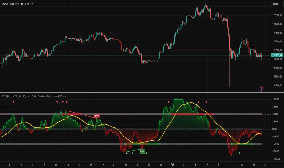
RSI Bollinger Bands [DCAUT]█ RSI Bollinger Bands
📊 ORIGINALITY & INNOVATION
The RSI Bollinger Bands indicator represents a meaningful advancement in momentum analysis by combining two proven technical tools: the Relative Strength Index (RSI) and Bollinger Bands. This combination addresses a significant limitation in traditional RSI analysis - the use of fixed overbought/oversold thresholds (typically 70/30) that fail to adapt to changing market volatility conditions.
Core Innovation:
Rather than relying on static threshold levels, this indicator applies Bollinger Bands statistical analysis directly to RSI values, creating dynamic zones that automatically adjust based on recent momentum volatility. This approach helps reduce false signals during low volatility periods while remaining sensitive to genuine extremes during high volatility conditions.
Key Enhancements Over Traditional RSI:
Dynamic Thresholds: Overbought/oversold zones adapt to market conditions automatically, eliminating the need for manual threshold adjustments across different instruments and timeframes
Volatility Context: Band width provides immediate visual feedback about momentum volatility, helping traders distinguish between stable trends and erratic movements
Reduced False Signals: During ranging markets, narrower bands filter out minor RSI fluctuations that would trigger traditional fixed-threshold signals
Breakout Preparation: Band squeeze patterns (similar to price-based BB) signal potential momentum regime changes before they occur
Self-Referencing Analysis: By measuring RSI against its own statistical behavior rather than arbitrary levels, the indicator provides more relevant context
📐 MATHEMATICAL FOUNDATION
Two-Stage Calculation Process:
Stage 1: RSI Calculation
RSI = 100 - (100 / (1 + RS))
where RS = Average Gain / Average Loss over specified period
The RSI normalizes price momentum into a bounded 0-100 scale, making it ideal for statistical band analysis.
Stage 2: Bollinger Bands on RSI
Basis = MA(RSI, BB Length)
Upper Band = Basis + (StdDev(RSI, BB Length) × Multiplier)
Lower Band = Basis - (StdDev(RSI, BB Length) × Multiplier)
Band Width = Upper Band - Lower Band
The Bollinger Bands measure RSI's standard deviation from its own moving average, creating statistically-derived dynamic zones.
Statistical Interpretation:
Under normal distribution assumptions with default 2.0 multiplier, approximately 95% of RSI values should fall within the bands
Band touches represent statistically significant momentum extremes relative to recent behavior
Band width expansion indicates increasing momentum volatility (strengthening trend or increasing uncertainty)
Band width contraction signals momentum consolidation and potential regime change preparation
📊 COMPREHENSIVE SIGNAL ANALYSIS
Visual Color Signals:
This indicator features dynamic color fills that highlight extreme momentum conditions:
Green Fill (Above Upper Band):
Appears when RSI breaks above the upper band, indicating exceptionally strong bullish momentum
Represents dynamic overbought zone - not necessarily a reversal signal but a warning of extreme conditions
In strong uptrends, green fills can persist as RSI "rides the band" - this indicates sustained momentum strength
Exit of green zone (RSI falling back below upper band) often signals initial momentum weakening
Red Fill (Below Lower Band):
Appears when RSI breaks below the lower band, indicating exceptionally weak bearish momentum
Represents dynamic oversold zone - potential reversal or continuation signal depending on trend context
In strong downtrends, red fills can persist as RSI "rides the band" - this indicates sustained selling pressure
Exit of red zone (RSI rising back above lower band) often signals initial momentum recovery
Position-Based Signals:
Upper Band Interactions:
RSI Touching Upper Band: Dynamic overbought condition - momentum is extremely strong relative to recent volatility, potential exhaustion or continuation depending on trend context
RSI Riding Upper Band: Sustained strong momentum, often seen in powerful trends, not necessarily an immediate reversal signal but warrants monitoring for exhaustion
RSI Crossing Below Upper Band: Initial momentum weakening signal, particularly significant if accompanied by price divergence
Lower Band Interactions:
RSI Touching Lower Band: Dynamic oversold condition - momentum is extremely weak relative to recent volatility, potential reversal or continuation of downtrend
RSI Riding Lower Band: Sustained weak momentum, common in strong downtrends, monitor for potential exhaustion
RSI Crossing Above Lower Band: Initial momentum strengthening signal, early indication of potential reversal or consolidation
Basis Line Signals:
RSI Above Basis: Bullish momentum regime - upward pressure dominant
RSI Below Basis: Bearish momentum regime - downward pressure dominant
Basis Crossovers: Momentum regime shifts, more significant when accompanied by band width changes
RSI Oscillating Around Basis: Balanced momentum, often indicates ranging market conditions
Volatility-Based Signals:
Band Width Patterns:
Narrow Bands (Squeeze): Momentum volatility compression, often precedes significant directional moves, similar to price coiling patterns
Expanding Bands: Increasing momentum volatility, indicates trend acceleration or growing uncertainty
Narrowest Band in 100 Bars: Extreme compression alert, high probability of upcoming volatility expansion
Advanced Pattern Recognition:
Divergence Analysis:
Bullish Divergence: Price makes lower lows while RSI touches or stays above previous lower band touch, suggests downward momentum weakening
Bearish Divergence: Price makes higher highs while RSI touches or stays below previous upper band touch, suggests upward momentum weakening
Hidden Bullish: Price makes higher lows while RSI makes lower lows at the lower band, indicates strong underlying bullish momentum
Hidden Bearish: Price makes lower highs while RSI makes higher highs at the upper band, indicates strong underlying bearish momentum
Band Walk Patterns:
Upper Band Walk: RSI consistently touching or staying near upper band indicates exceptionally strong trend, wait for clear break below basis before considering reversal
Lower Band Walk: RSI consistently at lower band signals very weak momentum, requires break above basis for reversal confirmation
🎯 STRATEGIC APPLICATIONS
Strategy 1: Mean Reversion Trading
Setup Conditions:
Market Type: Ranging or choppy markets with no clear directional trend
Timeframe: Works best on lower timeframes (5m-1H) or during consolidation phases
Band Characteristic: Normal to narrow band width
Entry Rules:
Long Entry: RSI touches or crosses below lower band, wait for RSI to start rising back toward basis before entry
Short Entry: RSI touches or crosses above upper band, wait for RSI to start falling back toward basis before entry
Confirmation: Use price action confirmation (candlestick reversal patterns) at band touches
Exit Rules:
Target: RSI returns to basis line or opposite band
Stop Loss: Fixed percentage or below recent swing low/high
Time Stop: Exit if position not profitable within expected timeframe
Strategy 2: Trend Continuation Trading
Setup Conditions:
Market Type: Clear trending market with higher highs/lower lows
Timeframe: Medium to higher timeframes (1H-Daily)
Band Characteristic: Expanding or wide bands indicating strong momentum
Entry Rules:
Long Entry in Uptrend: Wait for RSI to pull back to basis line or slightly below, enter when RSI starts rising again
Short Entry in Downtrend: Wait for RSI to rally to basis line or slightly above, enter when RSI starts falling again
Avoid Counter-Trend: Do not fade RSI at bands during strong trends (band walk patterns)
Exit Rules:
Trailing Stop: Move stop to break-even when RSI reaches opposite band
Trend Break: Exit when RSI crosses basis against trend direction with conviction
Band Squeeze: Reduce position size when bands start narrowing significantly
Strategy 3: Breakout Preparation
Setup Conditions:
Market Type: Consolidating market after significant move or at key technical levels
Timeframe: Any timeframe, but longer timeframes provide more reliable breakouts
Band Characteristic: Narrowest band width in recent 100 bars (squeeze alert)
Preparation Phase:
Identify band squeeze condition (bands at multi-period narrowest point)
Monitor price action for consolidation patterns (triangles, rectangles, flags)
Prepare bracket orders for both directions
Wait for band expansion to begin
Entry Execution:
Breakout Confirmation: Enter in direction of RSI band breakout (RSI breaks above upper band or below lower band)
Price Confirmation: Ensure price also breaks corresponding technical level
Volume Confirmation: Look for volume expansion supporting the breakout
Risk Management:
Stop Loss: Place beyond consolidation pattern opposite extreme
Position Sizing: Use smaller size due to false breakout risk
Quick Exit: Exit immediately if RSI returns inside bands within 1-3 bars
Strategy 4: Multi-Timeframe Analysis
Timeframe Selection:
Higher Timeframe: Daily or 4H for trend context
Trading Timeframe: 1H or 15m for entry signals
Confirmation Timeframe: 5m or 1m for precise entry timing
Analysis Process:
Trend Identification: Check higher timeframe RSI position relative to bands, trade only in direction of higher timeframe momentum
Setup Formation: Wait for trading timeframe RSI to show pullback to basis in trending direction
Entry Timing: Use confirmation timeframe RSI band touch or crossover for precise entry
Alignment Confirmation: All timeframes should show RSI moving in same direction for highest probability setups
📋 DETAILED PARAMETER CONFIGURATION
RSI Source:
Close (Default): Standard price point, balances responsiveness and reliability
HL2: Reduces noise from intrabar volatility, provides smoother RSI values
HLC3 or OHLC4: Further smoothing for very choppy markets, slower to respond but more stable
Volume-Weighted: Consider using VWAP or volume-weighted prices for additional liquidity context
RSI Length Parameter:
Shorter Periods (5-10): More responsive but generates more signals, suitable for scalping or very active trading, higher noise level
Standard (14): Default and most widely used setting, proven balance between responsiveness and reliability, recommended starting point
Longer Periods (21-30): Smoother momentum measurement, fewer but potentially more reliable signals, better for swing trading or position trading
Optimization Note: Test across different market regimes, optimal length often varies by instrument volatility characteristics
RSI MA Type Parameter:
RMA (Default): Wilder's original smoothing method, provides traditional RSI behavior with balanced lag, most widely recognized and tested, recommended for standard technical analysis
EMA: Exponential smoothing gives more weight to recent values, faster response to momentum changes, suitable for active trading and trending markets, reduces lag compared to RMA
SMA: Simple average treats all periods equally, smoothest output with highest lag, best for filtering noise in choppy markets, useful for long-term position analysis
WMA: Weighted average emphasizes recent data less aggressively than EMA, middle ground between SMA and EMA characteristics, balanced responsiveness for swing trading
Advanced Options: Full access to 25+ moving average types including HMA (reduced lag), DEMA/TEMA (enhanced responsiveness), KAMA/FRAMA (adaptive behavior), T3 (smoothness), Kalman Filter (optimal estimation)
Selection Guide: RMA for traditional analysis and backtesting consistency, EMA for faster signals in trending markets, SMA for stability in ranging markets, adaptive types (KAMA/FRAMA) for varying volatility regimes
BB Length Parameter:
Short Length (10-15): Tighter bands that react quickly to RSI changes, more frequent band touches, suitable for active trading styles
Standard (20): Balanced approach providing meaningful statistical context without excessive lag
Long Length (30-50): Smoother bands that filter minor RSI fluctuations, captures only significant momentum extremes, fewer but higher quality signals
Relationship to RSI Length: Consider BB Length greater than RSI Length for cleaner signals
BB MA Type Parameter:
SMA (Default): Standard Bollinger Bands calculation using simple moving average for basis line, treats all periods equally, widely recognized and tested approach
EMA: Exponential smoothing for basis line gives more weight to recent RSI values, creates more responsive bands that adapt faster to momentum changes, suitable for trending markets
RMA: Wilder's smoothing provides consistent behavior aligned with traditional RSI when using RMA for both RSI and BB calculations
WMA: Weighted average for basis line balances recent emphasis with historical context, middle ground between SMA and EMA responsiveness
Advanced Options: Full access to 25+ moving average types for basis calculation, including HMA (reduced lag), DEMA/TEMA (enhanced responsiveness), KAMA/FRAMA (adaptive to volatility changes)
Selection Guide: SMA for standard Bollinger Bands behavior and backtesting consistency, EMA for faster band adaptation in dynamic markets, matching RSI MA type creates unified smoothing behavior
BB Multiplier Parameter:
Conservative (1.5-1.8): Tighter bands resulting in more frequent touches, useful in low volatility environments, higher signal frequency but potentially more false signals
Standard (2.0): Default setting representing approximately 95% confidence interval under normal distribution, widely accepted statistical threshold
Aggressive (2.5-3.0): Wider bands capturing only extreme momentum conditions, fewer but potentially more significant signals, reduces false signals in high volatility
Adaptive Approach: Consider adjusting multiplier based on instrument characteristics, lower multiplier for stable instruments, higher for volatile instruments
Parameter Optimization Workflow:
Start with default parameters (RSI:14, BB:20, Mult:2.0)
Test across representative sample period including different market regimes
Adjust RSI length based on desired responsiveness vs stability tradeoff
Tune BB length to match your typical holding period
Modify multiplier to achieve desired signal frequency
Validate on out-of-sample data to avoid overfitting
Document optimal parameters for different instruments and timeframes
Reference Levels Display:
Enabled (Default): Shows traditional 30/50/70 levels for comparison with dynamic bands, helps visualize the adaptive advantage
Disabled: Cleaner chart focusing purely on dynamic zones, reduces visual clutter for experienced users
Educational Value: Keeping reference levels visible helps understand how dynamic bands differ from fixed thresholds across varying market conditions
📈 PERFORMANCE ANALYSIS & COMPETITIVE ADVANTAGES
Comparison with Traditional RSI:
Fixed Threshold RSI Limitations:
In ranging low-volatility markets: RSI rarely reaches 70/30, missing tradable extremes
In trending high-volatility markets: RSI frequently breaks through 70/30, generating excessive false reversal signals
Across different instruments: Same thresholds applied to volatile crypto and stable forex pairs produce inconsistent results
Threshold Adjustment Problem: Manually changing thresholds for different conditions is subjective and lagging
RSI Bollinger Bands Advantages:
Automatic Adaptation: Bands adjust to current volatility regime without manual intervention
Consistent Logic: Same statistical approach works across different instruments and timeframes
Reduced False Signals: Band width filtering helps distinguish meaningful extremes from noise
Additional Information: Band width provides volatility context missing in standard RSI
Objective Extremes: Statistical basis (standard deviations) provides objective extreme definition
Comparison with Price-Based Bollinger Bands:
Price BB Characteristics:
Measures absolute price volatility
Affected by large price gaps and outliers
Band position relative to price not normalized
Difficult to compare across different price scales
RSI BB Advantages:
Normalized Scale: RSI's 0-100 bounds make band interpretation consistent across all instruments
Momentum Focus: Directly measures momentum extremes rather than price extremes
Reduced Gap Impact: RSI calculation smooths price gaps impact on band calculations
Comparable Analysis: Same RSI BB appearance across stocks, forex, crypto enables consistent strategy application
Performance Characteristics:
Signal Quality:
Higher Signal-to-Noise Ratio: Dynamic bands help filter RSI oscillations that don't represent meaningful extremes
Context-Aware Alerts: Band width provides volatility context helping traders adjust position sizing and stop placement
Reduced Whipsaws: During consolidations, narrower bands prevent premature signals from minor RSI movements
Responsiveness:
Adaptive Lag: Band calculation introduces some lag, but this lag is adaptive to current conditions rather than fixed
Faster Than Manual Adjustment: Automatic band adjustment is faster than trader's ability to manually modify thresholds
Balanced Approach: Combines RSI's inherent momentum lag with BB's statistical smoothing for stable yet responsive signals
Versatility:
Multi-Strategy Application: Supports both mean reversion (ranging markets) and trend continuation (trending markets) approaches
Universal Instrument Coverage: Works effectively across equities, forex, commodities, cryptocurrencies without parameter changes
Timeframe Agnostic: Same interpretation applies from 1-minute charts to monthly charts
Limitations and Considerations:
Known Limitations:
Dual Lag Effect: Combines RSI's momentum lag with BB's statistical lag, making it less suitable for very short-term scalping
Requires Volatility History: Needs sufficient bars for BB calculation, less effective immediately after major regime changes
Statistical Assumptions: Assumes RSI values are somewhat normally distributed, extreme trending conditions may violate this
Not a Standalone System: Like all indicators, should be combined with price action analysis and risk management
Optimal Use Cases:
Best for swing trading and position trading timeframes
Most effective in markets with alternating volatility regimes
Ideal for traders who use multiple instruments and timeframes
Suitable for systematic trading approaches requiring consistent logic
Suboptimal Conditions:
Very low timeframes (< 5 minutes) where lag becomes problematic
Instruments with extreme volatility spikes (gap-prone markets)
Markets in strong persistent trends where mean reversion rarely occurs
Periods immediately following major structural changes (new trading regime)
USAGE NOTES
This indicator is designed for technical analysis and educational purposes to help traders understand the interaction between momentum measurement and statistical volatility bands. The RSI Bollinger Bands has limitations and should not be used as the sole basis for trading decisions.
Important Considerations:
No Predictive Guarantee: Past band touches and patterns do not guarantee future price behavior
Market Regime Dependency: Indicator performance varies significantly between trending and ranging market conditions
Complementary Analysis Required: Should be used alongside price action, support/resistance levels, and fundamental analysis
Risk Management Essential: Always use proper position sizing, stop losses, and risk controls regardless of signal quality
Parameter Sensitivity: Different instruments and timeframes may require parameter optimization for optimal results
Continuous Monitoring: Band characteristics change with market conditions, requiring ongoing assessment
Recommended Supporting Analysis:
Price structure analysis (support/resistance, trend lines)
Volume confirmation for breakout signals
Multiple timeframe alignment
Market context awareness (news events, session times)
Correlation analysis with related instruments
The indicator aims to provide adaptive momentum analysis that adjusts to changing market volatility, but traders must apply sound judgment, proper risk management, and comprehensive market analysis in their decision-making process.

Keltner Channel Enhanced [DCAUT]█ Keltner Channel Enhanced
📊 ORIGINALITY & INNOVATION
The Keltner Channel Enhanced represents an important advancement over standard Keltner Channel implementations by introducing dual flexibility in moving average selection for both the middle band and ATR calculation. While traditional Keltner Channels typically use EMA for the middle band and RMA (Wilder's smoothing) for ATR, this enhanced version provides access to 25+ moving average algorithms for both components, enabling traders to fine-tune the indicator's behavior to match specific market characteristics and trading approaches.
Key Advancements:
Dual MA Algorithm Flexibility: Independent selection of moving average types for middle band (25+ options) and ATR smoothing (25+ options), allowing optimization of both trend identification and volatility measurement separately
Enhanced Trend Sensitivity: Ability to use faster algorithms (HMA, T3) for middle band while maintaining stable volatility measurement with traditional ATR smoothing, or vice versa for different trading strategies
Adaptive Volatility Measurement: Choice of ATR smoothing algorithm affects channel responsiveness to volatility changes, from highly reactive (SMA, EMA) to smoothly adaptive (RMA, TEMA)
Comprehensive Alert System: Five distinct alert conditions covering breakouts, trend changes, and volatility expansion, enabling automated monitoring without constant chart observation
Multi-Timeframe Compatibility: Works effectively across all timeframes from intraday scalping to long-term position trading, with independent optimization of trend and volatility components
This implementation addresses key limitations of standard Keltner Channels: fixed EMA/RMA combination may not suit all market conditions or trading styles. By decoupling the trend component from volatility measurement and allowing independent algorithm selection, traders can create highly customized configurations for specific instruments and market phases.
📐 MATHEMATICAL FOUNDATION
Keltner Channel Enhanced uses a three-component calculation system that combines a flexible moving average middle band with ATR-based (Average True Range) upper and lower channels, creating volatility-adjusted trend-following bands.
Core Calculation Process:
1. Middle Band (Basis) Calculation:
The basis line is calculated using the selected moving average algorithm applied to the price source over the specified period:
basis = ma(source, length, maType)
Supported algorithms include EMA (standard choice, trend-biased), SMA (balanced and symmetric), HMA (reduced lag), WMA, VWMA, TEMA, T3, KAMA, and 17+ others.
2. Average True Range (ATR) Calculation:
ATR measures market volatility by calculating the average of true ranges over the specified period:
trueRange = max(high - low, abs(high - close ), abs(low - close ))
atrValue = ma(trueRange, atrLength, atrMaType)
ATR smoothing algorithm significantly affects channel behavior, with options including RMA (standard, very smooth), SMA (moderate smoothness), EMA (fast adaptation), TEMA (smooth yet responsive), and others.
3. Channel Calculation:
Upper and lower channels are positioned at specified multiples of ATR from the basis:
upperChannel = basis + (multiplier × atrValue)
lowerChannel = basis - (multiplier × atrValue)
Standard multiplier is 2.0, providing channels that dynamically adjust width based on market volatility.
Keltner Channel vs. Bollinger Bands - Key Differences:
While both indicators create volatility-based channels, they use fundamentally different volatility measures:
Keltner Channel (ATR-based):
Uses Average True Range to measure actual price movement volatility
Incorporates gaps and limit moves through true range calculation
More stable in trending markets, less prone to extreme compression
Better reflects intraday volatility and trading range
Typically fewer band touches, making touches more significant
More suitable for trend-following strategies
Bollinger Bands (Standard Deviation-based):
Uses statistical standard deviation to measure price dispersion
Based on closing prices only, doesn't account for intraday range
Can compress significantly during consolidation (squeeze patterns)
More touches in ranging markets
Better suited for mean-reversion strategies
Provides statistical probability framework (95% within 2 standard deviations)
Algorithm Combination Effects:
The interaction between middle band MA type and ATR MA type creates different indicator characteristics:
Trend-Focused Configuration (Fast MA + Slow ATR): Middle band uses HMA/EMA/T3, ATR uses RMA/TEMA, quick trend changes with stable channel width, suitable for trend-following
Volatility-Focused Configuration (Slow MA + Fast ATR): Middle band uses SMA/WMA, ATR uses EMA/SMA, stable trend with dynamic channel width, suitable for volatility trading
Balanced Configuration (Standard EMA/RMA): Classic Keltner Channel behavior, time-tested combination, suitable for general-purpose trend following
Adaptive Configuration (KAMA + KAMA): Self-adjusting indicator responding to efficiency ratio, suitable for markets with varying trend strength and volatility regimes
📊 COMPREHENSIVE SIGNAL ANALYSIS
Keltner Channel Enhanced provides multiple signal categories optimized for trend-following and breakout strategies.
Channel Position Signals:
Upper Channel Interaction:
Price Touching Upper Channel: Strong bullish momentum, price moving more than typical volatility range suggests, potential continuation signal in established uptrends
Price Breaking Above Upper Channel: Exceptional strength, price exceeding normal volatility expectations, consider adding to long positions or tightening trailing stops
Price Riding Upper Channel: Sustained strong uptrend, characteristic of powerful bull moves, stay with trend and avoid premature profit-taking
Price Rejection at Upper Channel: Momentum exhaustion signal, consider profit-taking on longs or waiting for pullback to middle band for reentry
Lower Channel Interaction:
Price Touching Lower Channel: Strong bearish momentum, price moving more than typical volatility range suggests, potential continuation signal in established downtrends
Price Breaking Below Lower Channel: Exceptional weakness, price exceeding normal volatility expectations, consider adding to short positions or protecting against further downside
Price Riding Lower Channel: Sustained strong downtrend, characteristic of powerful bear moves, stay with trend and avoid premature covering
Price Rejection at Lower Channel: Momentum exhaustion signal, consider covering shorts or waiting for bounce to middle band for reentry
Middle Band (Basis) Signals:
Trend Direction Confirmation:
Price Above Basis: Bullish trend bias, middle band acts as dynamic support in uptrends, consider long positions or holding existing longs
Price Below Basis: Bearish trend bias, middle band acts as dynamic resistance in downtrends, consider short positions or avoiding longs
Price Crossing Above Basis: Potential trend change from bearish to bullish, early signal to establish long positions
Price Crossing Below Basis: Potential trend change from bullish to bearish, early signal to establish short positions or exit longs
Pullback Trading Strategy:
Uptrend Pullback: Price pulls back from upper channel to middle band, finds support, and resumes upward, ideal long entry point
Downtrend Bounce: Price bounces from lower channel to middle band, meets resistance, and resumes downward, ideal short entry point
Basis Test: Strong trends often show price respecting the middle band as support/resistance on pullbacks
Failed Test: Price breaking through middle band against trend direction signals potential reversal
Volatility-Based Signals:
Narrow Channels (Low Volatility):
Consolidation Phase: Channels contract during periods of reduced volatility and directionless price action
Breakout Preparation: Narrow channels often precede significant directional moves as volatility cycles
Trading Approach: Reduce position sizes, wait for breakout confirmation, avoid range-bound strategies within channels
Breakout Direction: Monitor for price breaking decisively outside channel range with expanding width
Wide Channels (High Volatility):
Trending Phase: Channels expand during strong directional moves and increased volatility
Momentum Confirmation: Wide channels confirm genuine trend with substantial volatility backing
Trading Approach: Trend-following strategies excel, wider stops necessary, mean-reversion strategies risky
Exhaustion Signs: Extreme channel width (historical highs) may signal approaching consolidation or reversal
Advanced Pattern Recognition:
Channel Walking Pattern:
Upper Channel Walk: Price consistently touches or exceeds upper channel while staying above basis, very strong uptrend signal, hold longs aggressively
Lower Channel Walk: Price consistently touches or exceeds lower channel while staying below basis, very strong downtrend signal, hold shorts aggressively
Basis Support/Resistance: During channel walks, price typically uses middle band as support/resistance on minor pullbacks
Pattern Break: Price crossing basis during channel walk signals potential trend exhaustion
Squeeze and Release Pattern:
Squeeze Phase: Channels narrow significantly, price consolidates near middle band, volatility contracts
Direction Clues: Watch for price positioning relative to basis during squeeze (above = bullish bias, below = bearish bias)
Release Trigger: Price breaking outside narrow channel range with expanding width confirms breakout
Follow-Through: Measure squeeze height and project from breakout point for initial profit targets
Channel Expansion Pattern:
Breakout Confirmation: Rapid channel widening confirms volatility increase and genuine trend establishment
Entry Timing: Enter positions early in expansion phase before trend becomes overextended
Risk Management: Use channel width to size stops appropriately, wider channels require wider stops
Basis Bounce Pattern:
Clean Bounce: Price touches middle band and immediately reverses, confirms trend strength and entry opportunity
Multiple Bounces: Repeated basis bounces indicate strong, sustainable trend
Bounce Failure: Price penetrating basis signals weakening trend and potential reversal
Divergence Analysis:
Price/Channel Divergence: Price makes new high/low while staying within channel (not reaching outer band), suggests momentum weakening
Width/Price Divergence: Price breaks to new extremes but channel width contracts, suggests move lacks conviction
Reversal Signal: Divergences often precede trend reversals or significant consolidation periods
Multi-Timeframe Analysis:
Keltner Channels work particularly well in multi-timeframe trend-following approaches:
Three-Timeframe Alignment:
Higher Timeframe (Weekly/Daily): Identify major trend direction, note price position relative to basis and channels
Intermediate Timeframe (Daily/4H): Identify pullback opportunities within higher timeframe trend
Lower Timeframe (4H/1H): Time precise entries when price touches middle band or lower channel (in uptrends) with rejection
Optimal Entry Conditions:
Best Long Entries: Higher timeframe in uptrend (price above basis), intermediate timeframe pulls back to basis, lower timeframe shows rejection at middle band or lower channel
Best Short Entries: Higher timeframe in downtrend (price below basis), intermediate timeframe bounces to basis, lower timeframe shows rejection at middle band or upper channel
Risk Management: Use higher timeframe channel width to set position sizing, stops below/above higher timeframe channels
🎯 STRATEGIC APPLICATIONS
Keltner Channel Enhanced excels in trend-following and breakout strategies across different market conditions.
Trend Following Strategy:
Setup Requirements:
Identify established trend with price consistently on one side of basis line
Wait for pullback to middle band (basis) or brief penetration through it
Confirm trend resumption with price rejection at basis and move back toward outer channel
Enter in trend direction with stop beyond basis line
Entry Rules:
Uptrend Entry:
Price pulls back from upper channel to middle band, shows support at basis (bullish candlestick, momentum divergence)
Enter long on rejection/bounce from basis with stop 1-2 ATR below basis
Aggressive: Enter on first touch; Conservative: Wait for confirmation candle
Downtrend Entry:
Price bounces from lower channel to middle band, shows resistance at basis (bearish candlestick, momentum divergence)
Enter short on rejection/reversal from basis with stop 1-2 ATR above basis
Aggressive: Enter on first touch; Conservative: Wait for confirmation candle
Trend Management:
Trailing Stop: Use basis line as dynamic trailing stop, exit if price closes beyond basis against position
Profit Taking: Take partial profits at opposite channel, move stops to basis
Position Additions: Add to winners on subsequent basis bounces if trend intact
Breakout Strategy:
Setup Requirements:
Identify consolidation period with contracting channel width
Monitor price action near middle band with reduced volatility
Wait for decisive breakout beyond channel range with expanding width
Enter in breakout direction after confirmation
Breakout Confirmation:
Price breaks clearly outside channel (upper for longs, lower for shorts), channel width begins expanding from contracted state
Volume increases significantly on breakout (if using volume analysis)
Price sustains outside channel for multiple bars without immediate reversal
Entry Approaches:
Aggressive: Enter on initial break with stop at opposite channel or basis, use smaller position size
Conservative: Wait for pullback to broken channel level, enter on rejection and resumption, tighter stop
Volatility-Based Position Sizing:
Adjust position sizing based on channel width (ATR-based volatility):
Wide Channels (High ATR): Reduce position size as stops must be wider, calculate position size using ATR-based risk calculation: Risk / (Stop Distance in ATR × ATR Value)
Narrow Channels (Low ATR): Increase position size as stops can be tighter, be cautious of impending volatility expansion
ATR-Based Risk Management: Use ATR-based risk calculations, position size = 0.01 × Capital / (2 × ATR), use multiples of ATR (1-2 ATR) for adaptive stops
Algorithm Selection Guidelines:
Different market conditions benefit from different algorithm combinations:
Strong Trending Markets: Middle band use EMA or HMA, ATR use RMA, capture trends quickly while maintaining stable channel width
Choppy/Ranging Markets: Middle band use SMA or WMA, ATR use SMA or WMA, avoid false trend signals while identifying genuine reversals
Volatile Markets: Middle band and ATR both use KAMA or FRAMA, self-adjusting to changing market conditions reduces manual optimization
Breakout Trading: Middle band use SMA, ATR use EMA or SMA, stable trend with dynamic channels highlights volatility expansion early
Scalping/Day Trading: Middle band use HMA or T3, ATR use EMA or TEMA, both components respond quickly
Position Trading: Middle band use EMA/TEMA/T3, ATR use RMA or TEMA, filter out noise for long-term trend-following
📋 DETAILED PARAMETER CONFIGURATION
Understanding and optimizing parameters is essential for adapting Keltner Channel Enhanced to specific trading approaches.
Source Parameter:
Close (Most Common): Uses closing price, reflects daily settlement, best for end-of-day analysis and position trading, standard choice
HL2 (Median Price): Smooths out closing bias, better represents full daily range in volatile markets, good for swing trading
HLC3 (Typical Price): Gives more weight to close while including full range, popular for intraday applications, slightly more responsive than HL2
OHLC4 (Average Price): Most comprehensive price representation, smoothest option, good for gap-prone markets or highly volatile instruments
Length Parameter:
Controls the lookback period for middle band (basis) calculation:
Short Periods (10-15): Very responsive to price changes, suitable for day trading and scalping, higher false signal rate
Standard Period (20 - Default): Represents approximately one month of trading, good balance between responsiveness and stability, suitable for swing and position trading
Medium Periods (30-50): Smoother trend identification, fewer false signals, better for position trading and longer holding periods
Long Periods (50+): Very smooth, identifies major trends only, minimal false signals but significant lag, suitable for long-term investment
Optimization by Timeframe: 1-15 minute charts use 10-20 period, 30-60 minute charts use 20-30 period, 4-hour to daily charts use 20-40 period, weekly charts use 20-30 weeks.
ATR Length Parameter:
Controls the lookback period for Average True Range calculation, affecting channel width:
Short ATR Periods (5-10): Very responsive to recent volatility changes, standard is 10 (Keltner's original specification), may be too reactive in whipsaw conditions
Standard ATR Period (10 - Default): Chester Keltner's original specification, good balance between responsiveness and stability, most widely used
Medium ATR Periods (14-20): Smoother channel width, ATR 14 aligns with Wilder's original ATR specification, good for position trading
Long ATR Periods (20+): Very smooth channel width, suitable for long-term trend-following
Length vs. ATR Length Relationship: Equal values (20/20) provide balanced responsiveness, longer ATR (20/14) gives more stable channel width, shorter ATR (20/10) is standard configuration, much shorter ATR (20/5) creates very dynamic channels.
Multiplier Parameter:
Controls channel width by setting ATR multiples:
Lower Values (1.0-1.5): Tighter channels with frequent price touches, more trading signals, higher false signal rate, better for range-bound and mean-reversion strategies
Standard Value (2.0 - Default): Chester Keltner's recommended setting, good balance between signal frequency and reliability, suitable for both trending and ranging strategies
Higher Values (2.5-3.0): Wider channels with less frequent touches, fewer but potentially higher-quality signals, better for strong trending markets
Market-Specific Optimization: High volatility markets (crypto, small-caps) use 2.5-3.0 multiplier, medium volatility markets (major forex, large-caps) use 2.0 multiplier, low volatility markets (bonds, utilities) use 1.5-2.0 multiplier.
MA Type Parameter (Middle Band):
Critical selection that determines trend identification characteristics:
EMA (Exponential Moving Average - Default): Standard Keltner Channel choice, Chester Keltner's original specification, emphasizes recent prices, faster response to trend changes, suitable for all timeframes
SMA (Simple Moving Average): Equal weighting of all data points, no directional bias, slower than EMA, better for ranging markets and mean-reversion
HMA (Hull Moving Average): Minimal lag with smooth output, excellent for fast trend identification, best for day trading and scalping
TEMA (Triple Exponential Moving Average): Advanced smoothing with reduced lag, responsive to trends while filtering noise, suitable for volatile markets
T3 (Tillson T3): Very smooth with minimal lag, excellent for established trend identification, suitable for position trading
KAMA (Kaufman Adaptive Moving Average): Automatically adjusts speed based on market efficiency, slow in ranging markets, fast in trends, suitable for markets with varying conditions
ATR MA Type Parameter:
Determines how Average True Range is smoothed, affecting channel width stability:
RMA (Wilder's Smoothing - Default): J. Welles Wilder's original ATR smoothing method, very smooth, slow to adapt to volatility changes, provides stable channel width
SMA (Simple Moving Average): Equal weighting, moderate smoothness, faster response to volatility changes than RMA, more dynamic channel width
EMA (Exponential Moving Average): Emphasizes recent volatility, quick adaptation to new volatility regimes, very responsive channel width changes
TEMA (Triple Exponential Moving Average): Smooth yet responsive, good balance for varying volatility, suitable for most trading styles
Parameter Combination Strategies:
Conservative Trend-Following: Length 30/ATR Length 20/Multiplier 2.5, MA Type EMA or TEMA/ATR MA Type RMA, smooth trend with stable wide channels, suitable for position trading
Standard Balanced Approach: Length 20/ATR Length 10/Multiplier 2.0, MA Type EMA/ATR MA Type RMA, classic Keltner Channel configuration, suitable for general purpose swing trading
Aggressive Day Trading: Length 10-15/ATR Length 5-7/Multiplier 1.5-2.0, MA Type HMA or EMA/ATR MA Type EMA or SMA, fast trend with dynamic channels, suitable for scalping and day trading
Breakout Specialist: Length 20-30/ATR Length 5-10/Multiplier 2.0, MA Type SMA or WMA/ATR MA Type EMA or SMA, stable trend with responsive channel width
Adaptive All-Conditions: Length 20/ATR Length 10/Multiplier 2.0, MA Type KAMA or FRAMA/ATR MA Type KAMA or TEMA, self-adjusting to market conditions
Offset Parameter:
Controls horizontal positioning of channels on chart. Positive values shift channels to the right (future) for visual projection, negative values shift left (past) for historical analysis, zero (default) aligns with current price bars for real-time signal analysis. Offset affects only visual display, not alert conditions or actual calculations.
📈 PERFORMANCE ANALYSIS & COMPETITIVE ADVANTAGES
Keltner Channel Enhanced provides improvements over standard implementations while maintaining proven effectiveness.
Response Characteristics:
Standard EMA/RMA Configuration: Moderate trend lag (approximately 0.4 × length periods), smooth and stable channel width from RMA smoothing, good balance for most market conditions
Fast HMA/EMA Configuration: Approximately 60% reduction in trend lag compared to EMA, responsive channel width from EMA ATR smoothing, suitable for quick trend changes and breakouts
Adaptive KAMA/KAMA Configuration: Variable lag based on market efficiency, automatic adjustment to trending vs. ranging conditions, self-optimizing behavior reduces manual intervention
Comparison with Traditional Keltner Channels:
Enhanced Version Advantages:
Dual Algorithm Flexibility: Independent MA selection for trend and volatility vs. fixed EMA/RMA, separate tuning of trend responsiveness and channel stability
Market Adaptation: Choose configurations optimized for specific instruments and conditions, customize for scalping, swing, or position trading preferences
Comprehensive Alerts: Enhanced alert system including channel expansion detection
Traditional Version Advantages:
Simplicity: Fewer parameters, easier to understand and implement
Standardization: Fixed EMA/RMA combination ensures consistency across users
Research Base: Decades of backtesting and research on standard configuration
When to Use Enhanced Version: Trading multiple instruments with different characteristics, switching between trending and ranging markets, employing different strategies, algorithm-based trading systems requiring customization, seeking optimization for specific trading style and timeframe.
When to Use Standard Version: Beginning traders learning Keltner Channel concepts, following published research or trading systems, preferring simplicity and standardization, wanting to avoid optimization and curve-fitting risks.
Performance Across Market Conditions:
Strong Trending Markets: EMA or HMA basis with RMA or TEMA ATR smoothing provides quicker trend identification, pullbacks to basis offer excellent entry opportunities
Choppy/Ranging Markets: SMA or WMA basis with RMA ATR smoothing and lower multipliers, channel bounce strategies work well, avoid false breakouts
Volatile Markets: KAMA or FRAMA with EMA or TEMA, adaptive algorithms excel by automatic adjustment, wider multipliers (2.5-3.0) accommodate large price swings
Low Volatility/Consolidation: Channels narrow significantly indicating consolidation, algorithm choice less impactful, focus on detecting channel width contraction for breakout preparation
Keltner Channel vs. Bollinger Bands - Usage Comparison:
Favor Keltner Channels When: Trend-following is primary strategy, trading volatile instruments with gaps, want ATR-based volatility measurement, prefer fewer higher-quality channel touches, seeking stable channel width during trends.
Favor Bollinger Bands When: Mean-reversion is primary strategy, trading instruments with limited gaps, want statistical framework based on standard deviation, need squeeze patterns for breakout identification, prefer more frequent trading opportunities.
Use Both Together: Bollinger Band squeeze + Keltner Channel breakout is powerful combination, price outside Bollinger Bands but inside Keltner Channels indicates moderate signal, price outside both indicates very strong signal, Bollinger Bands for entries and Keltner Channels for trend confirmation.
Limitations and Considerations:
General Limitations:
Lagging Indicator: All moving averages lag price, even with reduced-lag algorithms
Trend-Dependent: Works best in trending markets, less effective in choppy conditions
No Direction Prediction: Indicates volatility and deviation, not future direction, requires confirmation
Enhanced Version Specific Considerations:
Optimization Risk: More parameters increase risk of curve-fitting historical data
Complexity: Additional choices may overwhelm beginning traders
Backtesting Challenges: Different algorithms produce different historical results
Mitigation Strategies:
Use Confirmation: Combine with momentum indicators (RSI, MACD), volume, or price action
Test Parameter Robustness: Ensure parameters work across range of values, not just optimized ones
Multi-Timeframe Analysis: Confirm signals across different timeframes
Proper Risk Management: Use appropriate position sizing and stops
Start Simple: Begin with standard EMA/RMA before exploring alternatives
Optimal Usage Recommendations:
For Maximum Effectiveness:
Start with standard EMA/RMA configuration to understand classic behavior
Experiment with alternatives on demo account or paper trading
Match algorithm combination to market condition and trading style
Use channel width analysis to identify market phases
Combine with complementary indicators for confirmation
Implement strict risk management using ATR-based position sizing
Focus on high-quality setups rather than trading every signal
Respect the trend: trade with basis direction for higher probability
Complementary Indicators:
RSI or Stochastic: Confirm momentum at channel extremes
MACD: Confirm trend direction and momentum shifts
Volume: Validate breakouts and trend strength
ADX: Measure trend strength, avoid Keltner signals in weak trends
Support/Resistance: Combine with traditional levels for high-probability setups
Bollinger Bands: Use together for enhanced breakout and volatility analysis
USAGE NOTES
This indicator is designed for technical analysis and educational purposes. Keltner Channel Enhanced has limitations and should not be used as the sole basis for trading decisions. While the flexible moving average selection for both trend and volatility components provides valuable adaptability across different market conditions, algorithm performance varies with market conditions, and past characteristics do not guarantee future results.
Key considerations:
Always use multiple forms of analysis and confirmation before entering trades
Backtest any parameter combination thoroughly before live trading
Be aware that optimization can lead to curve-fitting if not done carefully
Start with standard EMA/RMA settings and adjust only when specific conditions warrant
Understand that no moving average algorithm can eliminate lag entirely
Consider market regime (trending, ranging, volatile) when selecting parameters
Use ATR-based position sizing and risk management on every trade
Keltner Channels work best in trending markets, less effective in choppy conditions
Respect the trend direction indicated by price position relative to basis line
The enhanced flexibility of dual algorithm selection provides powerful tools for adaptation but requires responsible use, thorough understanding of how different algorithms behave under various market conditions, and disciplined risk management.

Opening Range IndicatorComplete Trading Guide: Opening Range Breakout Strategy
What Are Opening Ranges?
Opening ranges capture the high and low prices during the first few minutes of market open. These levels often act as key support and resistance throughout the trading day because:
Heavy volume occurs at market open as overnight orders execute
Institutional activity is concentrated during opening minutes
Price discovery happens as market participants react to overnight news
Psychological levels are established that traders watch all day
Understanding the Three Timeframes
OR5 (5-Minute Range: 9:30-9:35 AM)
Most sensitive - captures immediate market reaction
Quick signals but higher false breakout rate
Best for scalping and momentum trading
Use for early entry when conviction is high
OR15 (15-Minute Range: 9:30-9:45 AM)
Balanced approach - most popular among day traders
Moderate sensitivity with better reliability
Good for swing trades lasting several hours
Primary timeframe for most strategies
OR30 (30-Minute Range: 9:30-10:00 AM)
Most reliable but slower signals
Lower false breakout rate
Best for position trades and trend following
Use when looking for major moves
Core Trading Strategies
Strategy 1: Basic Breakout
Setup:
Wait for price to break above OR15 high or below OR15 low
Enter on the breakout candle close
Stop loss: Opposite side of the range
Target: 2-3x the range size
Example:
OR15 range: $100.00 - $102.00 (Range = $2.00)
Long entry: Break above $102.00
Stop loss: $99.50 (below OR15 low)
Target: $104.00+ (2x range size)
Strategy 2: Multiple Confirmation
Setup:
Wait for OR5 break first (early signal)
Confirm with OR15 break in same direction
Enter on OR15 confirmation
Stop: Below OR30 if available, or OR15 opposite level
Why it works:
Multiple timeframe confirmation reduces false signals and increases probability of sustained moves.
Strategy 3: Failed Breakout Reversal
Setup:
Price breaks OR15 level but fails to hold
Wait for re-entry into the range
Enter reversal trade toward opposite OR level
Stop: Recent breakout high/low
Target: Opposite side of range + extension
Key insight: Failed breakouts often lead to strong moves in the opposite direction.
Advanced Techniques
Range Quality Assessment
High-Quality Ranges (Trade these):
Range size: 0.5% - 2% of stock price
Clean boundaries (not choppy)
Volume spike during range formation
Clear rejection at range levels
Low-Quality Ranges (Avoid these):
Very narrow ranges (<0.3% of stock price)
Extremely wide ranges (>3% of stock price)
Choppy, overlapping candles
Low volume during formation
Volume Confirmation
For Breakouts:
Look for volume spike (2x+ average) on breakout
Declining volume often signals false breakout
Rising volume during range formation shows interest
Market Context Filters
Best Conditions:
Trending market days (SPY/QQQ with clear direction)
Earnings reactions or news-driven moves
High-volume stocks with good liquidity
Volatility above average (VIX considerations)
Avoid Trading When:
Extremely low volume days
Major economic announcements pending
Holidays or half-days
Choppy, sideways market conditions
Risk Management Rules
Position Sizing
Conservative: Risk 0.5% of account per trade
Moderate: Risk 1% of account per trade
Aggressive: Risk 2% maximum per trade
Stop Loss Placement
Inside the range: Quick exit but higher stop-out rate
Outside opposite level: More room but larger risk
ATR-based: 1.5-2x Average True Range below entry
Profit Taking
Target 1: 1x range size (take 50% off)
Target 2: 2x range size (take 25% off)
Runner: Trail remaining 25% with moving stops
Specific Entry Techniques
Breakout Entry Methods
Method 1: Immediate Entry
Enter as soon as price closes above/below range
Fastest entry but highest false signal rate
Best for strong momentum situations
Method 2: Pullback Entry
Wait for breakout, then pullback to range level
Enter when price bounces off former resistance/support
Better risk/reward but may miss some moves
Method 3: Volume Confirmation
Wait for breakout + volume spike
Enter after volume confirmation candle
Reduces false signals significantly
Multiple Timeframe Entries
Aggressive: OR5 break → immediate entry
Conservative: OR5 + OR15 + OR30 all align → enter
Balanced: OR15 break with OR30 support → enter
Common Mistakes to Avoid
1. Trading Poor-Quality Ranges
❌ Don't trade ranges that are too narrow or too wide
✅ Focus on clean, well-defined ranges with good volume
2. Ignoring Volume
❌ Don't chase breakouts without volume confirmation
✅ Always check for volume spike on breakouts
3. Over-Trading
❌ Don't force trades when ranges are unclear
✅ Wait for high-probability setups only
4. Poor Risk Management
❌ Don't risk more than planned or use tight stops in volatile conditions
✅ Stick to predetermined risk levels
5. Fighting the Trend
❌ Don't fade breakouts in strongly trending markets
✅ Align trades with overall market direction
Daily Trading Routine
Pre-Market (8:00-9:30 AM)
Check overnight news and earnings
Review major indices (SPY, QQQ, IWM)
Identify potential opening range candidates
Set alerts for range breakouts
Market Open (9:30-10:00 AM)
Watch opening range formation
Note volume and price action quality
Mark key levels on charts
Prepare for breakout signals
Trading Session (10:00 AM - 4:00 PM)
Execute breakout strategies
Manage existing positions
Trail stops as profits develop
Look for additional setups
Post-Market Review
Analyze winning and losing trades
Review range quality vs. outcomes
Identify improvement areas
Prepare for next session
Best Stocks/ETFs for Opening Range Trading
Large Cap Stocks (Best for beginners):
AAPL, MSFT, GOOGL, AMZN, TSLA
High liquidity, predictable behavior
Good range formation most days
ETFs (Consistent patterns):
SPY, QQQ, IWM, XLF, XLE
Excellent liquidity
Clear range boundaries
Mid-Cap Growth (Advanced traders):
Stocks with good volume (1M+ shares daily)
Recent news catalysts
Clean technical patterns
Performance Optimization
Track These Metrics:
Win rate by range type (OR5 vs OR15 vs OR30)
Average R/R (risk vs reward ratio)
Best performing market conditions
Time of day performance
Continuous Improvement:
Keep detailed trade journal
Review failed breakouts for patterns
Adjust position sizing based on win rate
Refine entry timing based on backtesting
Final Tips for Success
Start small - Paper trade or use tiny positions initially
Focus on quality - Better to miss trades than take bad ones
Stay disciplined - Stick to your rules even during losing streaks
Adapt to conditions - What works in trending markets may fail in choppy conditions
Keep learning - Markets evolve, so should your approach
The opening range strategy is powerful because it captures natural market behavior, but like all strategies, it requires practice, discipline, and proper risk management to be profitable long-term.

Small Business Economic Conditions - Statistical Analysis ModelThe Small Business Economic Conditions Statistical Analysis Model (SBO-SAM) represents an econometric approach to measuring and analyzing the economic health of small business enterprises through multi-dimensional factor analysis and statistical methodologies. This indicator synthesizes eight fundamental economic components into a composite index that provides real-time assessment of small business operating conditions with statistical rigor. The model employs Z-score standardization, variance-weighted aggregation, higher-order moment analysis, and regime-switching detection to deliver comprehensive insights into small business economic conditions with statistical confidence intervals and multi-language accessibility.
1. Introduction and Theoretical Foundation
The development of quantitative models for assessing small business economic conditions has gained significant importance in contemporary financial analysis, particularly given the critical role small enterprises play in economic development and employment generation. Small businesses, typically defined as enterprises with fewer than 500 employees according to the U.S. Small Business Administration, constitute approximately 99.9% of all businesses in the United States and employ nearly half of the private workforce (U.S. Small Business Administration, 2024).
The theoretical framework underlying the SBO-SAM model draws extensively from established academic research in small business economics and quantitative finance. The foundational understanding of key drivers affecting small business performance builds upon the seminal work of Dunkelberg and Wade (2023) in their analysis of small business economic trends through the National Federation of Independent Business (NFIB) Small Business Economic Trends survey. Their research established the critical importance of optimism, hiring plans, capital expenditure intentions, and credit availability as primary determinants of small business performance.
The model incorporates insights from Federal Reserve Board research, particularly the Senior Loan Officer Opinion Survey (Federal Reserve Board, 2024), which demonstrates the critical importance of credit market conditions in small business operations. This research consistently shows that small businesses face disproportionate challenges during periods of credit tightening, as they typically lack access to capital markets and rely heavily on bank financing.
The statistical methodology employed in this model follows the econometric principles established by Hamilton (1989) in his work on regime-switching models and time series analysis. Hamilton's framework provides the theoretical foundation for identifying different economic regimes and understanding how economic relationships may vary across different market conditions. The variance-weighted aggregation technique draws from modern portfolio theory as developed by Markowitz (1952) and later refined by Sharpe (1964), applying these concepts to economic indicator construction rather than traditional asset allocation.
Additional theoretical support comes from the work of Engle and Granger (1987) on cointegration analysis, which provides the statistical framework for combining multiple time series while maintaining long-term equilibrium relationships. The model also incorporates insights from behavioral economics research by Kahneman and Tversky (1979) on prospect theory, recognizing that small business decision-making may exhibit systematic biases that affect economic outcomes.
2. Model Architecture and Component Structure
The SBO-SAM model employs eight orthogonalized economic factors that collectively capture the multifaceted nature of small business operating conditions. Each component is normalized using Z-score standardization with a rolling 252-day window, representing approximately one business year of trading data. This approach ensures statistical consistency across different market regimes and economic cycles, following the methodology established by Tsay (2010) in his treatment of financial time series analysis.
2.1 Small Cap Relative Performance Component
The first component measures the performance of the Russell 2000 index relative to the S&P 500, capturing the market-based assessment of small business equity valuations. This component reflects investor sentiment toward smaller enterprises and provides a forward-looking perspective on small business prospects. The theoretical justification for this component stems from the efficient market hypothesis as formulated by Fama (1970), which suggests that stock prices incorporate all available information about future prospects.
The calculation employs a 20-day rate of change with exponential smoothing to reduce noise while preserving signal integrity. The mathematical formulation is:
Small_Cap_Performance = (Russell_2000_t / S&P_500_t) / (Russell_2000_{t-20} / S&P_500_{t-20}) - 1
This relative performance measure eliminates market-wide effects and isolates the specific performance differential between small and large capitalization stocks, providing a pure measure of small business market sentiment.
2.2 Credit Market Conditions Component
Credit Market Conditions constitute the second component, incorporating commercial lending volumes and credit spread dynamics. This factor recognizes that small businesses are particularly sensitive to credit availability and borrowing costs, as established in numerous Federal Reserve studies (Bernanke and Gertler, 1995). Small businesses typically face higher borrowing costs and more stringent lending standards compared to larger enterprises, making credit conditions a critical determinant of their operating environment.
The model calculates credit spreads using high-yield bond ETFs relative to Treasury securities, providing a market-based measure of credit risk premiums that directly affect small business borrowing costs. The component also incorporates commercial and industrial loan growth data from the Federal Reserve's H.8 statistical release, which provides direct evidence of lending activity to businesses.
The mathematical specification combines these elements as:
Credit_Conditions = α₁ × (HYG_t / TLT_t) + α₂ × C&I_Loan_Growth_t
where HYG represents high-yield corporate bond ETF prices, TLT represents long-term Treasury ETF prices, and C&I_Loan_Growth represents the rate of change in commercial and industrial loans outstanding.
2.3 Labor Market Dynamics Component
The Labor Market Dynamics component captures employment cost pressures and labor availability metrics through the relationship between job openings and unemployment claims. This factor acknowledges that labor market tightness significantly impacts small business operations, as these enterprises typically have less flexibility in wage negotiations and face greater challenges in attracting and retaining talent during periods of low unemployment.
The theoretical foundation for this component draws from search and matching theory as developed by Mortensen and Pissarides (1994), which explains how labor market frictions affect employment dynamics. Small businesses often face higher search costs and longer hiring processes, making them particularly sensitive to labor market conditions.
The component is calculated as:
Labor_Tightness = Job_Openings_t / (Unemployment_Claims_t × 52)
This ratio provides a measure of labor market tightness, with higher values indicating greater difficulty in finding workers and potential wage pressures.
2.4 Consumer Demand Strength Component
Consumer Demand Strength represents the fourth component, combining consumer sentiment data with retail sales growth rates. Small businesses are disproportionately affected by consumer spending patterns, making this component crucial for assessing their operating environment. The theoretical justification comes from the permanent income hypothesis developed by Friedman (1957), which explains how consumer spending responds to both current conditions and future expectations.
The model weights consumer confidence and actual spending data to provide both forward-looking sentiment and contemporaneous demand indicators. The specification is:
Demand_Strength = β₁ × Consumer_Sentiment_t + β₂ × Retail_Sales_Growth_t
where β₁ and β₂ are determined through principal component analysis to maximize the explanatory power of the combined measure.
2.5 Input Cost Pressures Component
Input Cost Pressures form the fifth component, utilizing producer price index data to capture inflationary pressures on small business operations. This component is inversely weighted, recognizing that rising input costs negatively impact small business profitability and operating conditions. Small businesses typically have limited pricing power and face challenges in passing through cost increases to customers, making them particularly vulnerable to input cost inflation.
The theoretical foundation draws from cost-push inflation theory as described by Gordon (1988), which explains how supply-side price pressures affect business operations. The model employs a 90-day rate of change to capture medium-term cost trends while filtering out short-term volatility:
Cost_Pressure = -1 × (PPI_t / PPI_{t-90} - 1)
The negative weighting reflects the inverse relationship between input costs and business conditions.
2.6 Monetary Policy Impact Component
Monetary Policy Impact represents the sixth component, incorporating federal funds rates and yield curve dynamics. Small businesses are particularly sensitive to interest rate changes due to their higher reliance on variable-rate financing and limited access to capital markets. The theoretical foundation comes from monetary transmission mechanism theory as developed by Bernanke and Blinder (1992), which explains how monetary policy affects different segments of the economy.
The model calculates the absolute deviation of federal funds rates from a neutral 2% level, recognizing that both extremely low and high rates can create operational challenges for small enterprises. The yield curve component captures the shape of the term structure, which affects both borrowing costs and economic expectations:
Monetary_Impact = γ₁ × |Fed_Funds_Rate_t - 2.0| + γ₂ × (10Y_Yield_t - 2Y_Yield_t)
2.7 Currency Valuation Effects Component
Currency Valuation Effects constitute the seventh component, measuring the impact of US Dollar strength on small business competitiveness. A stronger dollar can benefit businesses with significant import components while disadvantaging exporters. The model employs Dollar Index volatility as a proxy for currency-related uncertainty that affects small business planning and operations.
The theoretical foundation draws from international trade theory and the work of Krugman (1987) on exchange rate effects on different business segments. Small businesses often lack hedging capabilities, making them more vulnerable to currency fluctuations:
Currency_Impact = -1 × DXY_Volatility_t
2.8 Regional Banking Health Component
The eighth and final component, Regional Banking Health, assesses the relative performance of regional banks compared to large financial institutions. Regional banks traditionally serve as primary lenders to small businesses, making their health a critical factor in small business credit availability and overall operating conditions.
This component draws from the literature on relationship banking as developed by Boot (2000), which demonstrates the importance of bank-borrower relationships, particularly for small enterprises. The calculation compares regional bank performance to large financial institutions:
Banking_Health = (Regional_Banks_Index_t / Large_Banks_Index_t) - 1
3. Statistical Methodology and Advanced Analytics
The model employs statistical techniques to ensure robustness and reliability. Z-score normalization is applied to each component using rolling 252-day windows, providing standardized measures that remain consistent across different time periods and market conditions. This approach follows the methodology established by Engle and Granger (1987) in their cointegration analysis framework.
3.1 Variance-Weighted Aggregation
The composite index calculation utilizes variance-weighted aggregation, where component weights are determined by the inverse of their historical variance. This approach, derived from modern portfolio theory, ensures that more stable components receive higher weights while reducing the impact of highly volatile factors. The mathematical formulation follows the principle that optimal weights are inversely proportional to variance, maximizing the signal-to-noise ratio of the composite indicator.
The weight for component i is calculated as:
w_i = (1/σᵢ²) / Σⱼ(1/σⱼ²)
where σᵢ² represents the variance of component i over the lookback period.
3.2 Higher-Order Moment Analysis
Higher-order moment analysis extends beyond traditional mean and variance calculations to include skewness and kurtosis measurements. Skewness provides insight into the asymmetry of the sentiment distribution, while kurtosis measures the tail behavior and potential for extreme events. These metrics offer valuable information about the underlying distribution characteristics and potential regime changes.
Skewness is calculated as:
Skewness = E / σ³
Kurtosis is calculated as:
Kurtosis = E / σ⁴ - 3
where μ represents the mean and σ represents the standard deviation of the distribution.
3.3 Regime-Switching Detection
The model incorporates regime-switching detection capabilities based on the Hamilton (1989) framework. This allows for identification of different economic regimes characterized by distinct statistical properties. The regime classification employs percentile-based thresholds:
- Regime 3 (Very High): Percentile rank > 80
- Regime 2 (High): Percentile rank 60-80
- Regime 1 (Moderate High): Percentile rank 50-60
- Regime 0 (Neutral): Percentile rank 40-50
- Regime -1 (Moderate Low): Percentile rank 30-40
- Regime -2 (Low): Percentile rank 20-30
- Regime -3 (Very Low): Percentile rank < 20
3.4 Information Theory Applications
The model incorporates information theory concepts, specifically Shannon entropy measurement, to assess the information content of the sentiment distribution. Shannon entropy, as developed by Shannon (1948), provides a measure of the uncertainty or information content in a probability distribution:
H(X) = -Σᵢ p(xᵢ) log₂ p(xᵢ)
Higher entropy values indicate greater unpredictability and information content in the sentiment series.
3.5 Long-Term Memory Analysis
The Hurst exponent calculation provides insight into the long-term memory characteristics of the sentiment series. Originally developed by Hurst (1951) for analyzing Nile River flow patterns, this measure has found extensive application in financial time series analysis. The Hurst exponent H is calculated using the rescaled range statistic:
H = log(R/S) / log(T)
where R/S represents the rescaled range and T represents the time period. Values of H > 0.5 indicate long-term positive autocorrelation (persistence), while H < 0.5 indicates mean-reverting behavior.
3.6 Structural Break Detection
The model employs Chow test approximation for structural break detection, based on the methodology developed by Chow (1960). This technique identifies potential structural changes in the underlying relationships by comparing the stability of regression parameters across different time periods:
Chow_Statistic = (RSS_restricted - RSS_unrestricted) / RSS_unrestricted × (n-2k)/k
where RSS represents residual sum of squares, n represents sample size, and k represents the number of parameters.
4. Implementation Parameters and Configuration
4.1 Language Selection Parameters
The model provides comprehensive multi-language support across five languages: English, German (Deutsch), Spanish (Español), French (Français), and Japanese (日本語). This feature enhances accessibility for international users and ensures cultural appropriateness in terminology usage. The language selection affects all internal displays, statistical classifications, and alert messages while maintaining consistency in underlying calculations.
4.2 Model Configuration Parameters
Calculation Method: Users can select from four aggregation methodologies:
- Equal-Weighted: All components receive identical weights
- Variance-Weighted: Components weighted inversely to their historical variance
- Principal Component: Weights determined through principal component analysis
- Dynamic: Adaptive weighting based on recent performance
Sector Specification: The model allows for sector-specific calibration:
- General: Broad-based small business assessment
- Retail: Emphasis on consumer demand and seasonal factors
- Manufacturing: Enhanced weighting of input costs and currency effects
- Services: Focus on labor market dynamics and consumer demand
- Construction: Emphasis on credit conditions and monetary policy
Lookback Period: Statistical analysis window ranging from 126 to 504 trading days, with 252 days (one business year) as the optimal default based on academic research.
Smoothing Period: Exponential moving average period from 1 to 21 days, with 5 days providing optimal noise reduction while preserving signal integrity.
4.3 Statistical Threshold Parameters
Upper Statistical Boundary: Configurable threshold between 60-80 (default 70) representing the upper significance level for regime classification.
Lower Statistical Boundary: Configurable threshold between 20-40 (default 30) representing the lower significance level for regime classification.
Statistical Significance Level (α): Alpha level for statistical tests, configurable between 0.01-0.10 with 0.05 as the standard academic default.
4.4 Display and Visualization Parameters
Color Theme Selection: Eight professional color schemes optimized for different user preferences and accessibility requirements:
- Gold: Traditional financial industry colors
- EdgeTools: Professional blue-gray scheme
- Behavioral: Psychology-based color mapping
- Quant: Value-based quantitative color scheme
- Ocean: Blue-green maritime theme
- Fire: Warm red-orange theme
- Matrix: Green-black technology theme
- Arctic: Cool blue-white theme
Dark Mode Optimization: Automatic color adjustment for dark chart backgrounds, ensuring optimal readability across different viewing conditions.
Line Width Configuration: Main index line thickness adjustable from 1-5 pixels for optimal visibility.
Background Intensity: Transparency control for statistical regime backgrounds, adjustable from 90-99% for subtle visual enhancement without distraction.
4.5 Alert System Configuration
Alert Frequency Options: Three frequency settings to match different trading styles:
- Once Per Bar: Single alert per bar formation
- Once Per Bar Close: Alert only on confirmed bar close
- All: Continuous alerts for real-time monitoring
Statistical Extreme Alerts: Notifications when the index reaches 99% confidence levels (Z-score > 2.576 or < -2.576).
Regime Transition Alerts: Notifications when statistical boundaries are crossed, indicating potential regime changes.
5. Practical Application and Interpretation Guidelines
5.1 Index Interpretation Framework
The SBO-SAM index operates on a 0-100 scale with statistical normalization ensuring consistent interpretation across different time periods and market conditions. Values above 70 indicate statistically elevated small business conditions, suggesting favorable operating environment with potential for expansion and growth. Values below 30 indicate statistically reduced conditions, suggesting challenging operating environment with potential constraints on business activity.
The median reference line at 50 represents the long-term equilibrium level, with deviations providing insight into cyclical conditions relative to historical norms. The statistical confidence bands at 95% levels (approximately ±2 standard deviations) help identify when conditions reach statistically significant extremes.
5.2 Regime Classification System
The model employs a seven-level regime classification system based on percentile rankings:
Very High Regime (P80+): Exceptional small business conditions, typically associated with strong economic growth, easy credit availability, and favorable regulatory environment. Historical analysis suggests these periods often precede economic peaks and may warrant caution regarding sustainability.
High Regime (P60-80): Above-average conditions supporting business expansion and investment. These periods typically feature moderate growth, stable credit conditions, and positive consumer sentiment.
Moderate High Regime (P50-60): Slightly above-normal conditions with mixed signals. Careful monitoring of individual components helps identify emerging trends.
Neutral Regime (P40-50): Balanced conditions near long-term equilibrium. These periods often represent transition phases between different economic cycles.
Moderate Low Regime (P30-40): Slightly below-normal conditions with emerging headwinds. Early warning signals may appear in credit conditions or consumer demand.
Low Regime (P20-30): Below-average conditions suggesting challenging operating environment. Businesses may face constraints on growth and expansion.
Very Low Regime (P0-20): Severely constrained conditions, typically associated with economic recessions or financial crises. These periods often present opportunities for contrarian positioning.
5.3 Component Analysis and Diagnostics
Individual component analysis provides valuable diagnostic information about the underlying drivers of overall conditions. Divergences between components can signal emerging trends or structural changes in the economy.
Credit-Labor Divergence: When credit conditions improve while labor markets tighten, this may indicate early-stage economic acceleration with potential wage pressures.
Demand-Cost Divergence: Strong consumer demand coupled with rising input costs suggests inflationary pressures that may constrain small business margins.
Market-Fundamental Divergence: Disconnection between small-cap equity performance and fundamental conditions may indicate market inefficiencies or changing investor sentiment.
5.4 Temporal Analysis and Trend Identification
The model provides multiple temporal perspectives through momentum analysis, rate of change calculations, and trend decomposition. The 20-day momentum indicator helps identify short-term directional changes, while the Hodrick-Prescott filter approximation separates cyclical components from long-term trends.
Acceleration analysis through second-order momentum calculations provides early warning signals for potential trend reversals. Positive acceleration during declining conditions may indicate approaching inflection points, while negative acceleration during improving conditions may suggest momentum loss.
5.5 Statistical Confidence and Uncertainty Quantification
The model provides comprehensive uncertainty quantification through confidence intervals, volatility measures, and regime stability analysis. The 95% confidence bands help users understand the statistical significance of current readings and identify when conditions reach historically extreme levels.
Volatility analysis provides insight into the stability of current conditions, with higher volatility indicating greater uncertainty and potential for rapid changes. The regime stability measure, calculated as the inverse of volatility, helps assess the sustainability of current conditions.
6. Risk Management and Limitations
6.1 Model Limitations and Assumptions
The SBO-SAM model operates under several important assumptions that users must understand for proper interpretation. The model assumes that historical relationships between economic variables remain stable over time, though the regime-switching framework helps accommodate some structural changes. The 252-day lookback period provides reasonable statistical power while maintaining sensitivity to changing conditions, but may not capture longer-term structural shifts.
The model's reliance on publicly available economic data introduces inherent lags in some components, particularly those based on government statistics. Users should consider these timing differences when interpreting real-time conditions. Additionally, the model's focus on quantitative factors may not fully capture qualitative factors such as regulatory changes, geopolitical events, or technological disruptions that could significantly impact small business conditions.
The model's timeframe restrictions ensure statistical validity by preventing application to intraday periods where the underlying economic relationships may be distorted by market microstructure effects, trading noise, and temporal misalignment with the fundamental data sources. Users must utilize daily or longer timeframes to ensure the model's statistical foundations remain valid and interpretable.
6.2 Data Quality and Reliability Considerations
The model's accuracy depends heavily on the quality and availability of underlying economic data. Market-based components such as equity indices and bond prices provide real-time information but may be subject to short-term volatility unrelated to fundamental conditions. Economic statistics provide more stable fundamental information but may be subject to revisions and reporting delays.
Users should be aware that extreme market conditions may temporarily distort some components, particularly those based on financial market data. The model's statistical normalization helps mitigate these effects, but users should exercise additional caution during periods of market stress or unusual volatility.
6.3 Interpretation Caveats and Best Practices
The SBO-SAM model provides statistical analysis and should not be interpreted as investment advice or predictive forecasting. The model's output represents an assessment of current conditions based on historical relationships and may not accurately predict future outcomes. Users should combine the model's insights with other analytical tools and fundamental analysis for comprehensive decision-making.
The model's regime classifications are based on historical percentile rankings and may not fully capture the unique characteristics of current economic conditions. Users should consider the broader economic context and potential structural changes when interpreting regime classifications.
7. Academic References and Bibliography
Bernanke, B. S., & Blinder, A. S. (1992). The Federal Funds Rate and the Channels of Monetary Transmission. American Economic Review, 82(4), 901-921.
Bernanke, B. S., & Gertler, M. (1995). Inside the Black Box: The Credit Channel of Monetary Policy Transmission. Journal of Economic Perspectives, 9(4), 27-48.
Boot, A. W. A. (2000). Relationship Banking: What Do We Know? Journal of Financial Intermediation, 9(1), 7-25.
Chow, G. C. (1960). Tests of Equality Between Sets of Coefficients in Two Linear Regressions. Econometrica, 28(3), 591-605.
Dunkelberg, W. C., & Wade, H. (2023). NFIB Small Business Economic Trends. National Federation of Independent Business Research Foundation, Washington, D.C.
Engle, R. F., & Granger, C. W. J. (1987). Co-integration and Error Correction: Representation, Estimation, and Testing. Econometrica, 55(2), 251-276.
Fama, E. F. (1970). Efficient Capital Markets: A Review of Theory and Empirical Work. Journal of Finance, 25(2), 383-417.
Federal Reserve Board. (2024). Senior Loan Officer Opinion Survey on Bank Lending Practices. Board of Governors of the Federal Reserve System, Washington, D.C.
Friedman, M. (1957). A Theory of the Consumption Function. Princeton University Press, Princeton, NJ.
Gordon, R. J. (1988). The Role of Wages in the Inflation Process. American Economic Review, 78(2), 276-283.
Hamilton, J. D. (1989). A New Approach to the Economic Analysis of Nonstationary Time Series and the Business Cycle. Econometrica, 57(2), 357-384.
Hurst, H. E. (1951). Long-term Storage Capacity of Reservoirs. Transactions of the American Society of Civil Engineers, 116(1), 770-799.
Kahneman, D., & Tversky, A. (1979). Prospect Theory: An Analysis of Decision under Risk. Econometrica, 47(2), 263-291.
Krugman, P. (1987). Pricing to Market When the Exchange Rate Changes. In S. W. Arndt & J. D. Richardson (Eds.), Real-Financial Linkages among Open Economies (pp. 49-70). MIT Press, Cambridge, MA.
Markowitz, H. (1952). Portfolio Selection. Journal of Finance, 7(1), 77-91.
Mortensen, D. T., & Pissarides, C. A. (1994). Job Creation and Job Destruction in the Theory of Unemployment. Review of Economic Studies, 61(3), 397-415.
Shannon, C. E. (1948). A Mathematical Theory of Communication. Bell System Technical Journal, 27(3), 379-423.
Sharpe, W. F. (1964). Capital Asset Prices: A Theory of Market Equilibrium under Conditions of Risk. Journal of Finance, 19(3), 425-442.
Tsay, R. S. (2010). Analysis of Financial Time Series (3rd ed.). John Wiley & Sons, Hoboken, NJ.
U.S. Small Business Administration. (2024). Small Business Profile. Office of Advocacy, Washington, D.C.
8. Technical Implementation Notes
The SBO-SAM model is implemented in Pine Script version 6 for the TradingView platform, ensuring compatibility with modern charting and analysis tools. The implementation follows best practices for financial indicator development, including proper error handling, data validation, and performance optimization.
The model includes comprehensive timeframe validation to ensure statistical accuracy and reliability. The indicator operates exclusively on daily (1D) timeframes or higher, including weekly (1W), monthly (1M), and longer periods. This restriction ensures that the statistical analysis maintains appropriate temporal resolution for the underlying economic data sources, which are primarily reported on daily or longer intervals.
When users attempt to apply the model to intraday timeframes (such as 1-minute, 5-minute, 15-minute, 30-minute, 1-hour, 2-hour, 4-hour, 6-hour, 8-hour, or 12-hour charts), the system displays a comprehensive error message in the user's selected language and prevents execution. This safeguard protects users from potentially misleading results that could occur when applying daily-based economic analysis to shorter timeframes where the underlying data relationships may not hold.
The model's statistical calculations are performed using vectorized operations where possible to ensure computational efficiency. The multi-language support system employs Unicode character encoding to ensure proper display of international characters across different platforms and devices.
The alert system utilizes TradingView's native alert functionality, providing users with flexible notification options including email, SMS, and webhook integrations. The alert messages include comprehensive statistical information to support informed decision-making.
The model's visualization system employs professional color schemes designed for optimal readability across different chart backgrounds and display devices. The system includes dynamic color transitions based on momentum and volatility, professional glow effects for enhanced line visibility, and transparency controls that allow users to customize the visual intensity to match their preferences and analytical requirements. The clean confidence band implementation provides clear statistical boundaries without visual distractions, maintaining focus on the analytical content.

TRAPPER TRENDLINES — RSIBuilds dynamic RSI trendlines by connecting the two most recent confirmed RSI swing points (highs→highs for resistance, lows→lows for support). Includes optional channel shading for the 30–70 zone, an RSI moving average, clean break alerts, and simple bullish/bearish divergence alerts versus price.
How it works
RSI pivots: A point on RSI is a swing high/low only if it is the most extreme value compared with a set number of bars on the left and the right (the Pivot Lookback).
RSI trendlines:
Resistance connects the last two confirmed RSI swing highs.
Support connects the last two confirmed RSI swing lows.
Lines can be Full Extend (update into the future) or Pivot Only.
Channel block: Optional fill of the 30–70 range for fast visual context.
Alerts:
Breaks of RSI support/resistance trendlines.
Basic bullish/bearish RSI divergences versus price pivots.
Inputs
RSI
RSI Length: Default 14 (standard).
Pivot Lookback: Bars to the left/right required to confirm an RSI swing.
Overbought / Oversold: 70 / 30 by default.
Line Extension: Full Extend or Pivot Only.
Visuals
Show RSI Moving Average / Signal Length: Optional smoothing line on RSI.
RSI/Signal colors: Customize plot colors.
Show 30–70 Channel Block: Toggle the middle-zone fill.
Tint pane background when RSI in channel: Optional subtle background when RSI is between OB/OS.
Divergences & Alerts
Enable RSI TL Break Alerts: Alert conditions for RSI line breaks.
Enable Divergence Alerts: Bullish/Bearish divergence alerts versus price.
Pairing with price for confluence/divergence
For accurate confluence and clearer divergences, align this RSI tool with your price trendline tool (for example, TRAPPER TRENDLINES — PRICE):
Set RSI Pivot Lookback equal to the Pivot Left/Right size used on price.
Example: Price uses Pivot Left = 50 and Pivot Right = 50 → set RSI Pivot Lookback = 50.
Keep RSI Length = 14 and OB/OS = 70/30 unless you have a specific edge.
Interpretation:
Confluence: Price reacts at its trendline while RSI reacts at its own line in the same direction.
Divergence: Price makes a higher high while RSI makes a lower high (bearish), or price makes a lower low while RSI makes a higher low (bullish), using matched pivot windows.
Suggested settings
Higher timeframes (4H / 1D / 1W): Pivot Lookback = 50; optional RSI MA length 14; channel block ON.
Intraday (15m / 30m / 1H): Pivot Lookback = 30; optional RSI MA length 14.
Always mirror your price pivot size to this RSI Pivot Lookback for consistent swings.
Reading the signals
RSI trendline touch/hold: Momentum reacting at structure; look for confluence with price levels.
RSI Trendline Break Up / Down: Momentum shift; consider price structure and retests.
Bullish/Bearish Divergence: Confirm only when pivots are matched and the new swing is confirmed.
Notes & limitations
Pivots require future bars to confirm by design; trendlines update as new swings confirm.
Divergence logic compares RSI pivots to price pivots with the same lookback; mismatched windows can produce false positives.
No strategy entries/exits or performance claims are provided. This is an analytical tool.
Alerts (titles/messages)
RSI: Trendline Break Up — “RSI broke falling resistance line.”
RSI: Trendline Break Down — “RSI broke rising support line.”
RSI: Bullish Divergence — “Bullish RSI divergence confirmed.”
RSI: Bearish Divergence — “Bearish RSI divergence confirmed.”
Quick start
Add the indicator to a separate pane.
Set Pivot Lookback to match your price tool’s pivot size (e.g., 50).
Optionally toggle the RSI MA and Channel Block for clarity.
Enable alerts if you want notifications on RSI line breaks and divergences.
Use with TRAPPER TRENDLINES — PRICE or any price-based trendline tool for confluence/divergence analysis.
Compliance
This script is for educational purposes only and does not constitute financial advice. Trading involves risk. Past performance does not guarantee future results. No performance claims are made.

RTH Levels: VWAP + PDH/PDL + ONH/ONL + IBAlgo Index — Levels Pro (ONH/ONL • PDH/PDL • VWAP±Bands • IB • Gaps)
Purpose. A session-aware, non-repainting levels tool for intraday decision-making. Designed for futures and indices, with clean visuals, alerts, and a one-click Minimal Mode for screenshot-ready charts.
What it plots
• PDH/PDL (RTH-only) – Prior Regular Trading Hours high/low, computed intraday and frozen at the RTH close (no 24h mix-ups, no repainting).
• ONH/ONL – Prior Overnight high/low, held throughout RTH.
• RTH VWAP with ±σ bands – Volume-weighted variance, reset each RTH.
• Initial Balance (IB) – First N minutes of RTH, plus 1.5× / 2.0× extensions after IB completes.
• Today’s RTH Open & Prior RTH Close – With gap detection and “gap filled” alert.
• Killzone shading – NY Open (09:30–10:30 ET) and Lunch (11:15–13:30 ET).
• Values panel (top-right) – Each level with live distance in points & ticks.
• Right-edge level tags – With anti-overlap (stagger + vertical jitter).
• Price-scale tags – Native trackprice markers that always “stick” to the axis.
⸻
New in v6.4
• Minimal Mode: one click for a clean look (thinner lines, VWAP bands/IB extensions hidden, on-chart right-edge labels off; price-scale tags remain).
• Theme presets: Dark Hi-Contrast / Light Minimal / Futures Classic / Muted Dark.
• Anti-overlap controls: horizontal staggering, vertical jitter, and baseline offset to keep tags readable even when levels cluster.
⸻
Quick start (2 minutes)
1. Add to chart → keep defaults.
2. Sessions (ET):
• RTH Session default: 09:30–16:00 (US equities cash hours).
• Overnight Session default: 18:00–09:29.
Adjust for your market if you use different “day” hours (e.g., many use 08:20–13:30 ET for COMEX Gold).
3. Theme & Minimal Mode: pick a Theme Preset; enable Minimal Mode for screenshots.
4. Visibility: toggle PD/ON/VWAP/IB/References/Panel to taste.
5. Right-edge labels: turn Show Right-Edge Labels on. If they crowd, tune:
• Anti-overlap: min separation (ticks)
• Horizontal offset per tag (bars)
• Vertical jitter per step (ticks)
• Right-edge baseline offset (bars)
6. Alerts: open Add alert → Condition: and pick the events you want.
⸻
How levels are computed (no repainting)
• PDH/PDL: Intraday H/L are accumulated only while in RTH and saved at RTH close for “yesterday’s” values.
• ONH/ONL: Accumulated across the defined Overnight window and then held during RTH.
• RTH VWAP & ±σ: Volume-weighted mean and standard deviation, reset at the RTH open.
• IB: First N minutes of RTH (default 60). Extensions (1.5×/2.0×) appear after IB completes.
• Gaps: Today’s RTH open vs prior RTH close; “Gap Filled” triggers when price trades back to prior close.
⸻
Practical playbooks (how to trade around the levels)
1) PDH/PDL interactions
• Rejection: Price taps PDH/PDL then closes back inside → mean-reversion toward VWAP/IB.
• Acceptance: Close/hold beyond PDH/PDL with momentum → continuation to next HTF/IB target.
• Alert: PD Touch/Break.
2) ONH/ONL “taken”
• Often one ON extreme is taken during RTH. ONH Taken / ONL Taken → check if it’s a clean break or sweep & reclaim.
• Sweep + reclaim near VWAP can fuel rotations through the ON range.
3) VWAP ±σ framework
• Balanced: First tag of ±1σ often reverts toward VWAP.
• Trend: Persistent trade beyond ±1σ + IB break → target ±2σ/±3σ.
• Alerts: VWAP Cross and VWAP Reject (cross then immediate fail back).
4) IB breaks
• After IB completes, a clean IB break commonly targets 1.5× and sometimes 2.0×.
• Quick return inside IB = possible fade back to the opposite IB edge/VWAP.
• Alerts: IB Break Up / Down.
5) Gaps
• Gap-and-go: Opening drive away from prior close + VWAP support → trend until IB completion.
• Gap-fill: Weak open and VWAP overhead/underfoot → trade toward prior close; manage on Gap Filled alert.
Pro tip: Stack confluences (e.g., ONL sweep + VWAP reclaim + IB hold) and respect your execution rules (e.g., require a 5-minute close in direction, or your order-flow confirmation).
⸻
Inputs you’ll actually touch
• Sessions (ET): Session Timezone, RTH Session, Overnight Session.
• Visibility: toggles for PD/ON/VWAP/IB/Ref/Panel.
• VWAP bands: set σ multipliers (±1/±2/±3).
• IB: duration (minutes) and extension multipliers (1.5× / 2.0×).
• Style & Theme: Theme Preset, Main Line Width, Trackprice, Minimal Mode, and anti-overlap controls.
⸻
Alerts included
• PD Touch/Break — High ≥ PDH or Low ≤ PDL
• ONH Taken / ONL Taken — First in-RTH take of ONH/ONL
• VWAP Cross — Close crosses VWAP
• VWAP Reject — Cross then immediate fail back
• IB Break Up / Down — Break of IB High/Low after IB completes
• Gap Filled — Price trades back to prior RTH close
Setup: Add alert → Condition: Algo Index — Levels Pro → choose event → message → Notify on app/email.
⸻
Panel guide
The top-right panel shows each level plus live distance from last price:
LevelValue (Δpoints | Δticks)
Coloring: green if level is below current price, red if above.
⸻
Styling & screenshot tips
• Use Theme Preset that matches your chart.
• For dark charts, “Dark Hi-Contrast” with Main Line Width = 3 works well.
• Enable Trackprice for crisp axis tags that always stick to the right edge.
• Turn on Minimal Mode for cleaner screenshots (no VWAP bands or IB extensions, on-chart tags off; price-scale tags remain).
• If tags crowd, increase min separation (ticks) to 30–60 and horizontal offset to 3–5; add vertical jitter (4–12 ticks) and/or push tags farther right with baseline offset (bars).
⸻
Behavior & limitations
• Levels are computed incrementally; tables refresh on the last bar for efficiency.
• Right-edge labels are placed at bar_index + offset and do not track extra right-margin scrolling (TradingView limitation). The price-scale tags (from trackprice) do track the axis.
• “RTH” is what you define in inputs. If your market uses different day hours, change the session strings so PDH/PDL reflect your definition of “yesterday’s session.”
⸻
FAQ
Q: My PDH/PDL don’t match the daily chart.
A: By design this uses RTH-only highs/lows, not 24h daily bars. Adjust sessions if you want a different definition.
Q: Right-edge tags overlap or don’t sit at the far right.
A: Increase min separation / horizontal offset / vertical jitter and/or push tags farther with baseline offset. If you want markers that always hug the axis, rely on Trackprice.
Q: Can I change killzones?
A: Yes—edit the session strings in settings or request a version with user inputs for custom windows.
⸻
Disclaimer
Educational use only. This is not financial advice. Always apply your own risk management and confirmation rules.
⸻
Enjoy it? Please ⭐ the script and share screenshots using Minimal Mode + a Theme Preset that fits your style.
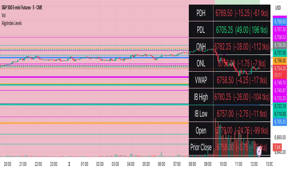
Monthly Expected Move (IV + Realized)What it does
Overlays 1-month expected move bands on price using both forward-looking options data and backward-looking realized movement:
IV30 band — from your pasted 30-day implied vol (%)
Straddle band — from your pasted ATM ~30-DTE call+put total
HV band — from Historical Volatility computed on-chart
ATR band — from ATR% extrapolated to ~1 trading month
Use it to quickly answer: “How much could this stock move in ~1 month?” and “Is the market now pricing more/less movement than we’ve actually been getting?”
Inputs (quick)
Implied (forward-looking)
Use IV30 (%) — paste annualized IV30 from your options platform.
Use ATM 30-DTE Straddle — paste Call+Put total (per share) at the ATM strike, ~30 DTE.
Realized (backward-looking)
HV lookback (days) — default 21 (≈1 trading month).
ATR length — default 14.
Note: TradingView can’t fetch option data automatically. Paste the IV30 % or the straddle total you read from your broker (use Mark/mid prices).
How it’s calculated
IV band (±%) = IV30 × √(21/252) (annualized → ~1-month).
Straddle band (±%) = (ATM Call + Put) / Spot to that expiry (≈30 DTE).
HV band (±%) = stdev(log returns, N) × √252 × √(21/252).
ATR band (±%) = (ATR(len)/Close) × √21.
All bands are plotted as upper/lower envelopes around price, plus an on-chart readout of each ±% for quick scanning.
How to use it (at a glance)
IV/Straddle bands wider than HV/ATR → market expects bigger movement than recent actuals (possible catalyst/expansion).
All bands narrow → likely a low-mover; look elsewhere if you want action.
HV > IV → realized swings exceed current pricing (mean-reversion or vol bleed often follows).
Pro tips
For ATM straddle: pick the expiry closest to ~30 DTE, use the ATM strike (closest to spot), and add Call Mark + Put Mark (per share). If the exact ATM strike isn’t quoted, average the two neighboring strikes.
The simple straddle/spot heuristic can read slightly below the IV-derived 1σ; that’s normal.
Keep the chart on daily timeframe—the math assumes trading-day conventions (~252/yr, ~21/mo).
NY HIGH LOW BREAKNY HIGH LOW BREAK: A New York Session Breakout Strategy
The "NY HIGH LOW BREAK" indicator is a powerful TradingView script designed to identify and capitalize on breakout opportunities during the New York trading session. This strategy focuses on the initial price action of the New York market open, looking for clear breaches of the high or low established within the first 30 minutes. It's particularly suited for intraday traders who seek to capture momentum-driven moves.
Strategy Logic
The core of the "NY HIGH LOW BREAK" strategy revolves around these key components:
New York Session Opening Range Identification:
The script first identifies the opening range of the New York session. This is defined by the high and low prices established during the first 30 minutes of the New York trading session (from 7:01 AM GMT-4 to 7:31 AM GMT-4).
These crucial levels are then extended forward on the chart as horizontal lines, serving as potential support and resistance zones.
Breakout Signal Generation:
Long Signal: A buy signal is generated when the price breaks above the high of the New York opening range. Specifically, it looks for a candle whose open and close are both above the highLinePrice, and importantly, the previous candle's open was below and close was above the highLinePrice. This indicates a strong upward momentum confirming the breakout.
Short Signal: Conversely, a sell signal is generated when the price breaks below the low of the New York opening range. It looks for a candle whose open and close are both below the lowLinePrice, and the previous candle's open was above and close was below the lowLinePrice. This suggests strong downward momentum confirming the breakdown.
Supertrend Filter (Implicit/Future Enhancement):
While the supertrend and direction variables are present in the code, they are not actively used in the current signal generation logic. This suggests a potential future enhancement where the Supertrend indicator could be incorporated as a trend filter to confirm breakout directions, adding an extra layer of confluence to the signals. For example, only taking long breakouts when Supertrend indicates an uptrend, and short breakouts when Supertrend indicates a downtrend.
Second Candle Confirmation (Possible Future Enhancement):
The close_sec_candle function and openSEC, closeSEC variables indicate an attempt to capture the open and close of a "second candle" (30 minutes after the initial New York open). Currently, closeSEC is used in a specific condition for signal_way but not directly in the primary longSignal or shortSignal logic. This also suggests a potential future refinement where the price action of this second candle could be used for further confirmation or specific entry criteria.
Time-Based Filtering:
Signals are only considered valid within a specific trading window from 8:00 AM GMT-4 to 8:00 AM GMT-4 + 16 * 30 minutes (which is 480 minutes, or 8 hours) on 1-minute and 5-minute timeframes. This ensures that trades are taken during the most active and volatile periods of the New York session, avoiding late-session chop.
The script also highlights the New York session and lunch hours using background colors, providing visual context to the trading day.
Key Features
Automated New York Open Range Detection: The script automatically identifies and plots the high and low of the first 30 minutes of the New York trading session.
Clear Breakout Signals: Visually distinct "BUY" and "SELL" labels appear on the chart when a breakout occurs, making it easy to spot trading opportunities.
Timeframe Adaptability: While optimized for 1-minute and 5-minute timeframes for signal generation, the opening range lines can be displayed on various timeframes.
Customizable Risk-to-Reward (RR): The rr input allows users to define their preferred risk-to-reward ratio for potential trades, although it's not directly implemented in the current signal or trade management logic. This could be used by traders for manual trade management.
Visual Session and Lunch Highlights: The script colors the background to clearly delineate the New York trading session and the lunch break, helping traders understand the market context.
How to Use
Apply the Indicator: Add the "NY HIGH LOW BREAK" indicator to your chart on TradingView.
Select a Relevant Timeframe: For optimal signal generation, use 1-minute or 5-minute timeframes.
Observe the Opening Range: The green and red lines represent the high and low of the first 30 minutes of the New York session.
Look for Breakouts: Wait for price to decisively break above the green line (for a buy) or below the red line (for a sell).
Confirm Signals: The "BUY" or "SELL" labels will appear on the chart when the breakout conditions are met within the active trading window.
Implement Your Risk Management: Use your preferred risk management techniques, including stop-loss and take-profit levels, in conjunction with the signals generated. The rr input can guide your manual risk-to-reward calculations.
Potential Enhancements & Considerations
Supertrend Confirmation: Integrating the supertrend variable to filter signals would significantly enhance the strategy's robustness by aligning trades with the prevailing trend.
Stop-Loss and Take-Profit Automation: The rr input currently serves as a manual guide. Future versions could integrate automated stop-loss and take-profit placement based on this ratio, potentially using ATR for dynamic sizing.
Volume Confirmation: Adding a volume filter to confirm breakouts would ensure that only high-conviction moves are traded.
Backtesting and Optimization: Thorough backtesting across various assets and market conditions is crucial to determine the optimal settings and profitability of this strategy.
Session Times: The current session times are hardcoded. Making these user-definable inputs would allow for greater flexibility across different time zones and trading preferences.
The "NY HIGH LOW BREAK" is a straightforward yet effective strategy for capturing initial New York session momentum. By focusing on clear breakout levels, it aims to provide timely and actionable trading signals for intraday traders.

Profitable Loser Model [MMT]Profitable Loser Model
Overview
The Profitable Loser Model is a powerful PineScript v6 indicator designed to enhance your trading by visualizing key price levels, session open zones, Fibonacci retracements, and premium/discount zones. This overlay indicator provides traders with a customizable toolkit to analyze market structure across any timeframe, making it ideal for intraday and swing trading strategies.
Features
Open Zone Visualization
- Plots a box based on the open and close of the first candle in a user-defined timeframe (default: 5-minute).
- Customizable box color, projection offset, and label size (Tiny, Small, Normal, Large).
- Displays a timeframe label (e.g., "5m Open Zone") for quick reference, toggleable on/off.
Session Open Lines
- Optionally draws horizontal lines at key session opens (8:30 AM, 9:30 AM, 1:30 PM, Midnight, New York time).
- Customize line color, style (Solid, Dashed, Dotted), width, and label size for each session.
- Perfect for identifying critical intraday price levels.
Premium and Discount Zones
- Highlights premium (above midpoint) and discount (below midpoint) zones based on session high/low.
- Toggleable with customizable colors and projection offsets.
- Helps traders spot overbought/oversold areas for potential mean-reversion trades.
Fibonacci Retracement Levels
- Plots user-defined Fibonacci levels (default: 0.23, 0.35, 0.5, 0.62, 0.705, 0.79, 0.886, 1, 1.1).
- Customizable line style, width, color, and labels (showing percentage and/or price).
- Dynamically adjusts based on price movement relative to the open zone.
Take Profit (TP) and Stop Loss (SL) Levels
- Highlights TP (default: 0.23) and SL (default: 1.1) Fibonacci levels with distinct colors.
- Fully customizable to align with your risk-reward strategy.
How It Works
- Session Detection : Resets daily (or per user-defined timeframe) to capture the first candle's open, high, low, and close.
- Open Zone : Draws a box between the open and close, extended forward by the projection offset.
- Session Lines : Plots lines at specified session opens with customizable styles and labels.
- Fibonacci Retracement : Adjusts levels dynamically based on session high/low and price action.
- Premium/Discount Zones : Calculated from the session range midpoint, updated in real-time.
Settings
- Open Zone :
- Timeframe (default: 5m), Calculate Timeframe (default: Daily).
- Toggle label, adjust size, box color, and projection offset.
- Session Open Lines :
- Enable/disable lines for 8:30 AM, 9:30 AM, 1:30 PM, Midnight.
- Customize color, style, width, label size, and vertical offset.
- Premium/Discount Zones :
- Toggle visibility, set colors, and adjust projection offset.
- Fibonacci Retracement :
- Toggle visibility, set custom levels, line style, width, color, and label options.
- Adjust projection offset.
- TP/SL :
- Set TP/SL Fibonacci levels and colors.
Use Cases
- Intraday Trading : Use session open lines and open zones to trade key market hours.
- Swing Trading : Leverage Fibonacci levels for potential reversal or continuation zones.
- Risk Management : Set precise TP/SL levels based on Fibonacci retracements.
- Market Structure : Identify overbought/oversold zones with premium/discount areas.
Notes
- Optimized with `dynamic_requests = true` for efficient real-time data handling.
- Visual elements (boxes, lines, labels) are cleaned up at the start of each new session.
- Session lines use New York time (`America/New_York`) for alignment with major markets.
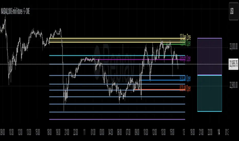
GeeksDoByte 15m & 30m ORB + Prev Day High/LowCME_MINI:NQ1!
How It Works
Opening Ranges
At 9:30 ET, the script begins tracking the high & low.
It uses two fixed sessions:
15 min from 09:30 to 09:45
30 min from 09:30 to 10:00
On the very first bar of each session it initializes the range, then continuously updates the high/low on each new intraday bar.
Dashed lines are drawn when the session opens and extended horizontally across subsequent bars.
Previous Day’s Levels
Independently, it fetches yesterday’s high and low via a daily security call.
These historic levels are plotted as simple horizontal lines for daily context.
How to Use
Breakout Entries
A close above the 15 min ORB high can signal an early breakout; a further push above the 30 min ORB high confirms extended momentum.
Conversely, breaks below the respective lows can indicate short setups.
Support & Resistance
Yesterday’s high/low often act as magnet levels. If price is near the previous high when the opening ranges break, you get a confluence zone worth watching.
Trade Management
Combine the two opening-range levels to tier your stops or scale in.
For example, you might place an initial stop below the 15 min low and a wider stop below the 30 min low.
