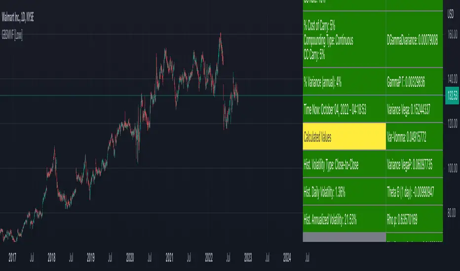
Moneyness Options [Loxx]A moneyness option is basically a plain vanilla option where the strike is set to a percentage of the future/forward price. For example, a 120% moneyness call would have a strike equal to 120% of the forward price. A 120% moneyness put would have a spot equal to 120% of the strike. The value of this option is given in percent of the forward. The value of a moneyness call or put is thus given by: (via "The Complete Guide to Option Pricing Formulas")
c = p = c^-rT * (N(d1) - LN(d2))
where L = X/F for a call and L = F/X for a put, and
d1 = (-log(L) + v^2*T/2) / (v*T^0.5)
d2 = d1 - (v*T^0.5)
b=r options on non-dividend paying stock
b=r-q options on stock or index paying a dividend yield of q
b=0 options on futures
b=r-rf currency options (where rf is the rate in the second currency)
Inputs
S = Stock price.
K = Strike price of option.
T = Time to expiration in years.
r = Risk-free rate
c = Cost of Carry
V = Variance of the underlying asset price
lambda = Jump rate per year
cnd1(x) = Cumulative Normal Distribution
nd(x) = Standard Normal Density Function
convertingToCCRate(r, cmp ) = Rate compounder
Numerical Greeks or Greeks by Finite Difference
Analytical Greeks are the standard approach to estimating Delta, Gamma etc... That is what we typically use when we can derive from closed form solutions. Normally, these are well-defined and available in text books. Previously, we relied on closed form solutions for the call or put formulae differentiated with respect to the Black Scholes parameters. When Greeks formulae are difficult to develop or tease out, we can alternatively employ numerical Greeks - sometimes referred to finite difference approximations. A key advantage of numerical Greeks relates to their estimation independent of deriving mathematical Greeks. This could be important when we examine American options where there may not technically exist an exact closed form solution that is straightforward to work with. (via VinegarHill FinanceLabs)
Things to know
Only works on the daily timeframe and for the current source price.
You can adjust the text size to fit the screen
Buscar en scripts para "technical"

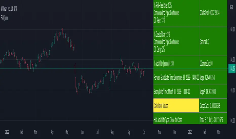
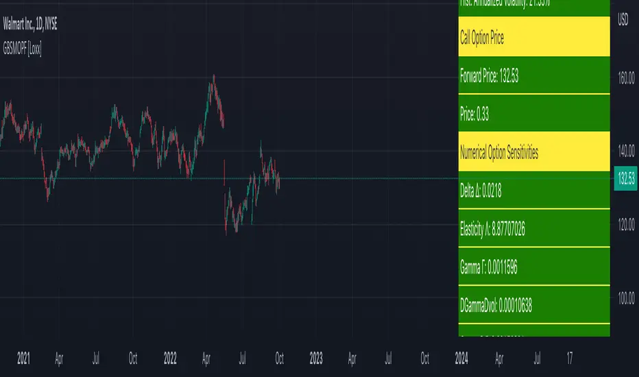
Forward Start Options [Loxx]A forward start option with time to maturity T starts at-the-money or proportionally in- or out-of-the-money after a known elapsed time t in the future. The strike is set equal to a positive constant a times the asset price S after the known time t. If a is less than unity, the call (put) will start 1 - a percent in-the-money (out-of-the- money); if a is unity, the option will start at-the-money; and if a is larger than unity, the call (put) will start a - 1 percentage out-of-the- money (in-the-money).A forward start option can be priced using the Rubinstein (1990) formula: (via "The Complete Guide to Option Pricing Formulas")
c = S*e^(b-r)t * (e^(b-r)(T-t) * N(d1)) - alpha * e^-r(T-t) * N(d2))
p = S*e^(b-r)t * (alpha*e^r(T-t) * N(-d2)) - e^-(b-r)(T-t) * N(-d1))
where
d1 = (log(1/alpha) + (b + v^2/2)(T-1))/v*(T-t)^0.5
d2 = d1 - v*(T-t)^0.5
Application
Employee options are often of the forward starting type. Ratchet options (aka cliquet options) consist of a series of forward starting options.
b=r options on non-dividend paying stock
b=r-q options on stock or index paying a dividend yield of q
b=0 options on futures
b=r-rf currency options (where rf is the rate in the second currency)
Inputs
S = Stock price.
a = Alpha
T1 = Time to forward start
T = Time to expiration in years.
r = Risk-free rate
c = Cost of Carry
v = volatility of the underlying asset price
Numerical Greeks or Greeks by Finite Difference
Analytical Greeks are the standard approach to estimating Delta, Gamma etc... That is what we typically use when we can derive from closed form solutions. Normally, these are well-defined and available in text books. Previously, we relied on closed form solutions for the call or put formulae differentiated with respect to the Black Scholes parameters. When Greeks formulae are difficult to develop or tease out, we can alternatively employ numerical Greeks - sometimes referred to finite difference approximations. A key advantage of numerical Greeks relates to their estimation independent of deriving mathematical Greeks. This could be important when we examine American options where there may not technically exist an exact closed form solution that is straightforward to work with. (via VinegarHill FinanceLabs)
Things to know
Only works on the daily timeframe and for the current source price.
You can adjust the text size to fit the screen
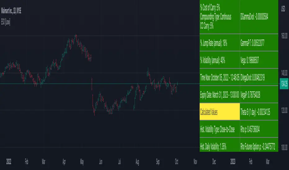
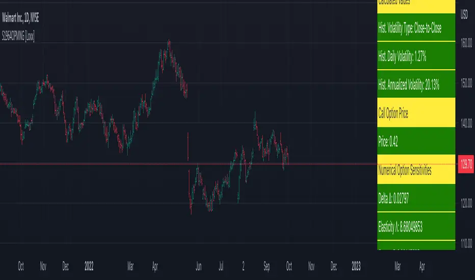
Executive Stock Options [Loxx]The Jennergren and Naslund (1993) formula takes into account that an employee or executive often loses her options if she has to leave the company before the option's expiration: (via "The Complete Guide to Option Pricing Formulas")
c = e^(-lambda*T) * (Se^((b-r)T) * N(d1) - Xe^-rT * N(d2))
p = e^(-lambda*T) * (Xe^(-rT) * N(-d2) - Se^(b-r)T * N(-d1))
where
d1 = (log(S/X) + (b + v^2/2)T) / vT^0.5
d2 = d1 - vT^0.5
lambda is the jump rate per year. The value of the executive option equals the ordinary Black-Scholes option price multiplied by the probability e —AT that the executive will stay with the firm until the option expires.
b=r options on non-dividend paying stock
b=r-q options on stock or index paying a dividend yield of q
b=0 options on futures
b=r-rf currency options (where rf is the rate in the second currency)
Inputs
S = Stock price.
K = Strike price of option.
T = Time to expiration in years.
r = Risk-free rate
c = Cost of Carry
V = Variance of the underlying asset price
lambda = Jump rate per year
cnd1(x) = Cumulative Normal Distribution
nd(x) = Standard Normal Density Function
convertingToCCRate(r, cmp ) = Rate compounder
Numerical Greeks or Greeks by Finite Difference
Analytical Greeks are the standard approach to estimating Delta, Gamma etc... That is what we typically use when we can derive from closed form solutions. Normally, these are well-defined and available in text books. Previously, we relied on closed form solutions for the call or put formulae differentiated with respect to the Black Scholes parameters. When Greeks formulae are difficult to develop or tease out, we can alternatively employ numerical Greeks - sometimes referred to finite difference approximations. A key advantage of numerical Greeks relates to their estimation independent of deriving mathematical Greeks. This could be important when we examine American options where there may not technically exist an exact closed form solution that is straightforward to work with. (via VinegarHill FinanceLabs)
Things to know
Only works on the daily timeframe and for the current source price.
You can adjust the text size to fit the screen
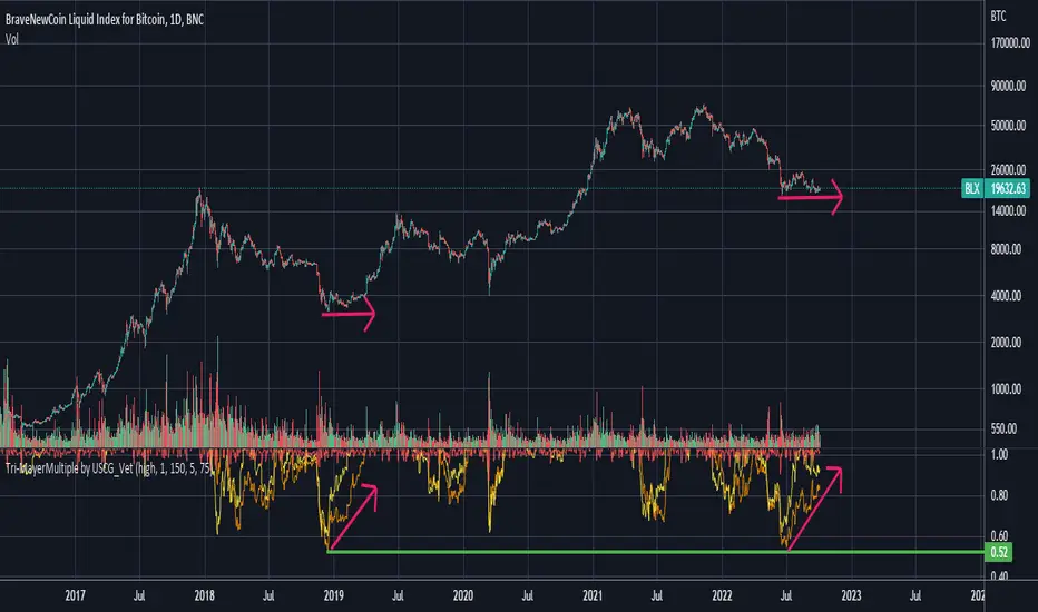
Tri-MayerMultiple by USCG_VetThe Mayer Multiple was created by Trace Mayer as a way to analyze the price of an asset in a historical context.
The Mayer Multiple is the multiple of the current price over some x-day moving average.
I preferred to display multiple average lines as they can help with identifying divergences.
Perpetual American Options [Loxx]Perpetual American Options is Perpetual American Options pricing model. This indicator also includes numerical greeks.
American Perpetual Options
While there in general is no closed-form solution for American options (except for non-dividend-paying stock call options) it is possible to find a closed-form solution for options with an infinite time to expiration. The reason is that the time to expiration will always be the same: infinite. The time to maturity, therefore, does not depend on at what point in time we look at the valuation problem, which makes the valuation problem independent of time McKean (1965) and Merton (1973) gives closed-form solutions for American perpetual options. For a call option we have
c = (X / (y1 - 1)) * ((y1 - 1)/y1 * S/X)^y1
where
y1 = 1/2 - b/v^2 + ((b/v^2 - 1/2)^2 + 2*r/v^2)^0.5
If b >= r, then there is never optimal to exercise a call option. In the case of an American perpetual put, we have
p = X/(1-y2) * (((y2 - 1) / y2) * S/X)^y2
where
y2 = 1/2 - b/v^2 - ((b/v^2 - 1/2)^2 + 2*r/v^2)^0.5
In practice, one can naturally discuss if there is such a thing as infinite time to maturity. For instance, credit risk could play an important role: Even when you are buying an option from an AAA bank, there is no guarantee the bank will be around forever.
b=r options on non-dividend paying stock
b=r-q options on stock or index paying a dividend yield of q
b=0 options on futures
b=r-rf currency options (where rf is the rate in the second currency)
Inputs
S = Stock price.
K = Strike price of option.
T = Time to expiration in years.
r = Risk-free rate
c = Cost of Carry
V = Variance of the underlying asset price
cnd1(x) = Cumulative Normal Distribution
cbnd3(x) = Cumulative Bivariate Normal Distribution
nd(x) = Standard Normal Density Function
convertingToCCRate(r, cmp ) = Rate compounder
Numerical Greeks or Greeks by Finite Difference
Analytical Greeks are the standard approach to estimating Delta, Gamma etc... That is what we typically use when we can derive from closed form solutions. Normally, these are well-defined and available in text books. Previously, we relied on closed form solutions for the call or put formulae differentiated with respect to the Black Scholes parameters. When Greeks formulae are difficult to develop or tease out, we can alternatively employ numerical Greeks - sometimes referred to finite difference approximations. A key advantage of numerical Greeks relates to their estimation independent of deriving mathematical Greeks. This could be important when we examine American options where there may not technically exist an exact closed form solution that is straightforward to work with. (via VinegarHill FinanceLabs)
Things to know
Only works on the daily timeframe and for the current source price.
You can adjust the text size to fit the screen
American Approximation Bjerksund & Stensland 2002 [Loxx]American Approximation Bjerksund & Stensland 2002 is an American Options pricing model. This indicator also includes numerical greeks. You can compare the output of the American Approximation to the Black-Scholes-Merton value on the output of the options panel.
The Bjerksund & Stensland (2002) Approximation
The Bjerksund and Stensland (2002) approximation divides the time to maturity into two parts, each with a separate flat exercise boundary. It is thus a straightforward generalization of the Bjerksund-Stensland 1993 algorithm. The method is fast and efficient and should be more accurate than the Barone-Adesi and Whaley (1987) and the Bjerksund and Stensland (1993b) approximations. The algorithm requires an accurate cumulative bivariate normal approximation. Several approximations that are described in the literature are not sufficiently accurate, but the Genze algorithm works.
C = alpha2*S^B - alpha2*phi(S, t1, B, I2, I2)
+ phi(S, t1, I2, I2) - phi(S, t1, I, I1, I2)
- X*phi(S, t1, 0, I2, I2) + X*phi(S, t1, 0, I1, I2)
+ alpha1*phi(X, t1, B, I1, I2) - alpha1*psi*St, T, B, I1, I2, I1, t1)
+ psi(S, T, 1, I1, I2, I1, t1) - psi(S, T, 1, X, I2, I1, t1)
- X*psi(S, T, 0, I1, I2, I1, t1) + psi(S, T, 0 ,X, I2, I1, t1)
where
alpha1 = (I1 - X)*I1^-B
alpha2 = (I2 - X)*I2^-B
B = (1/2 - b/v^2) + ((b/v^2 - 1/2)^2 + 2*(r/v^2))^0.5
The function psi(S, T, y, H, I) is given by
psi(S, T, gamma, H, I) = e^lambda * S^gamma * (N(-d) - (I/S)^k * N(-d2))
d = (log(S/H) + (b + (gamma - 1/2) * v^2) * T) / (v * T^0.5)
d2 = (log(I^2/(S*H)) + (b + (gamma - 1/2) * v^2) * T) / (v * T^0.5)
lambda = -r + gamma * b + 1/2 * gamma * (gamma - 1) * v^2
k = 2*b/v^2 + (2 * gamma - 1)
and the trigger price I is defined as
I1 = B0 + (B(+infi) - B0) * (1 - e^h1)
I2 = B0 + (B(+infi) - B0) * (1 - e^h2)
h1 = -(b*t1 + 2*v*t1^0.5) * (X^2 / ((B(+infi) - B0))*B0)
h2 = -(b*T + 2*v*T^0.5) * (X^2 / ((B(+infi) - B0))*B0)
t1 = 1/2 * (5^0.5 - 1) * T
B(+infi) = (B / (B - 1)) * X
B0 = max(X, (r / (r - b)) * X)
Moreover, the function psi(S, T, gamma, H, I2, I1, t1) is given by
psi(S, T, gamma, H, I2, I1, t1, r, b, v) = e^(lambda * T) * S^gamma * (M(-e1, -f1, rho) - (I2/S)^k * M(-e2, -f2, rho)
- (I1/S)^k * M(-e3, -f3, -rho) + (I1/I2)^k * M(-e4, -f4, -rho))
where (see screenshot for e and f values)
b=r options on non-dividend paying stock
b=r-q options on stock or index paying a dividend yield of q
b=0 options on futures
b=r-rf currency options (where rf is the rate in the second currency)
Inputs
S = Stock price.
K = Strike price of option.
T = Time to expiration in years.
r = Risk-free rate
c = Cost of Carry
V = Variance of the underlying asset price
cnd1(x) = Cumulative Normal Distribution
cbnd3(x) = Cumulative Bivariate Normal Distribution
nd(x) = Standard Normal Density Function
convertingToCCRate(r, cmp ) = Rate compounder
Numerical Greeks or Greeks by Finite Difference
Analytical Greeks are the standard approach to estimating Delta, Gamma etc... That is what we typically use when we can derive from closed form solutions. Normally, these are well-defined and available in text books. Previously, we relied on closed form solutions for the call or put formulae differentiated with respect to the Black Scholes parameters. When Greeks formulae are difficult to develop or tease out, we can alternatively employ numerical Greeks - sometimes referred to finite difference approximations. A key advantage of numerical Greeks relates to their estimation independent of deriving mathematical Greeks. This could be important when we examine American options where there may not technically exist an exact closed form solution that is straightforward to work with. (via VinegarHill FinanceLabs)
Things to know
Only works on the daily timeframe and for the current source price.
You can adjust the text size to fit the screen

American Approximation Bjerksund & Stensland 1993 [Loxx]American Approximation Bjerksund & Stensland 1993 is an American Options pricing model. This indicator also includes numerical greeks. You can compare the output of the American Approximation to the Black-Scholes-Merton value on the output of the options panel.
The Bjerksund and Stensland (1993) approximation can be used to price American options on stocks, futures, and currencies. The method is analytical and extremely computer-efficient. Bjerksund and Stensland's approximation is based on an exercise strategy corresponding to a flat boundary / (trigger price). Numerical investigation indicates that the Bjerksund and Stensland model is somewhat more accurate for long-term options than the Barone-Adesi and Whaley model. (The Complete Guide to Option Pricing Formulas)
C = alpha * X^beta - alpha Ø(S, T, beta, I, I) + Ø(S, T, I, I, I) - Ø(S, T, I, X, I) - XØ(S, T, 0, I, I) + XØ(S, T, 0, X, I)
where
alpha = (1 - X) * I^-beta
beta = (1/2 - b/v^2) + ((b/v^2 - 1/2)^2 + 2*(r/v^2))^0.5
The function Ø(S, T, y, H, I) is given by
Ø(S, T, gamma, H, I) = e^lambda * S^gamma * (N(d) - (I/S)^k * N(d - (2 * log(I/S)) / v*T^0.5))
lambda = (-r + gamma * b + 1/2 * gamma(gamma - 1) * v^2) * T
d = (log(S/H) + (b + (gamma - 1/2) * v^2) * T) / (v * T^0.5)
k = 2*b/v^2 + (2 * gamma - 1)
and the trigger price I is defined as
I = B0 + (B(+infi) - B0) * (1 - e^h(T))
h(T) = -(b*T + 2*v*T^0.5) * (B0 / (B(+infi) - B0))
B(+infi) = (B / (B - 1)) * X
B0 = max(X, (r / (r - b)) * X)
If s > I, it is optimal to exercise the option immediately, and the value must be equal to the intrinsic value of S - X. On the other hand, if b > r, it will never be optimal to exercise the American call option before expiration, and the value can be found using the generalized BSM formula. The value of the American put is given by the Bjerksund and Stensland put-call transformation
P(S, X, T, r, b, v) = C(X, S, T, r -b, -b, v)
where C(*) is the value of the American call with risk-free rate r - b and drift -b. With the use of this transformation, it is not necessary to develop a separate formula for an American put option.
b=r options on non-dividend paying stock
b=r-q options on stock or index paying a dividend yield of q
b=0 options on futures
b=r-rf currency options (where rf is the rate in the second currency)
Inputs
S = Stock price.
K = Strike price of option.
T = Time to expiration in years.
r = Risk-free rate
c = Cost of Carry
V = Variance of the underlying asset price
cnd1(x) = Cumulative Normal Distribution
cbnd3(x) = Cumulative Bivariate Normal Distribution
nd(x) = Standard Normal Density Function
convertingToCCRate(r, cmp ) = Rate compounder
Numerical Greeks or Greeks by Finite Difference
Analytical Greeks are the standard approach to estimating Delta, Gamma etc... That is what we typically use when we can derive from closed form solutions. Normally, these are well-defined and available in text books. Previously, we relied on closed form solutions for the call or put formulae differentiated with respect to the Black Scholes parameters. When Greeks formulae are difficult to develop or tease out, we can alternatively employ numerical Greeks - sometimes referred to finite difference approximations. A key advantage of numerical Greeks relates to their estimation independent of deriving mathematical Greeks. This could be important when we examine American options where there may not technically exist an exact closed form solution that is straightforward to work with. (via VinegarHill FinanceLabs)
Things to know
Only works on the daily timeframe and for the current source price.
You can adjust the text size to fit the screen
[blackcat] L3 Candle Skew 3821 TraderLevel 3
Background
By modeling skew to produce long and short entry points.
Function
The concept of skew comes from physics and statistics, and is used in market technical analysis to reflect the expectation of future stock price distribution. Because the return distribution of stocks in the trend market has skew (Skew), it is reasonable to judge the trend continuity according to the historical and current skew. It is precisely because the stock price rises that there is a skew. The greater the strength of the rise, the greater the angle of inclination and the greater the skew. The degree of this upward or downward slope in the statistical distribution of stock prices is defined as skew. Through the size of skew, we can know the direction, inertia and extent of the stock's rise or fall, and find stocks with a high probability of quick profit. The technical indicator introduced today is a simplified but effective stock price skew model used to generate buying and selling points.
The principle of this technical indicator is based on the success rate test results of different moving averages corresponding to different skews as follows:
10 trading cycles profit 5% success rate (%)
5 period moving average 10 period moving average 20 period moving average 30 period moving average 60 period moving average
skew>=0 51.36 52.26 52.65 52.55 52.08
skew>=0.5 55.44 58.06 60.56 62.37 65.66
skew>=1 59.72 63.06 67.07 69.78 70.62
skew>=1.5 63.01 67.08 71.61 72.9 70.61
skew>=2 65.53 70.22 74.18 73.76 70.12
skew>=2.5 67.89 72.93 75.32 73.66 68.92
skew>=3 70.07 75.32 75.69 72.54 67.45
skew>=3.5 71.85 77.05 75.32 73.63 63.82
skew>=4 73.6 78.06 74.19 68.96 59.91
skew>=4.5 76.04 78.56 72.85 69.55 49.24
skew>=5 77.44 78.88 71.58 67.28 51.69
skew>=5.5 78.97 78.39 70.33 64.31 49.7
skew>=6 79.68 78.07 68.82 61.65 53.57
Table 1
As can be seen from the above table, with the increase of the 5-period and 10-period moving average skew values, the success rate is increasing, but after the 20- and 30-period moving average skew values increase to an upper bound, it shows a downward trend. When the skew of the 20-period and 30-period moving averages is greater than 0.5, the 10-period profit of 5% is above 60%, and when it is greater than 1.5, the success rate can reach above 70%. The larger the 5-period moving average skew, the higher the success rate, but often because the short-term skew is too large, the stock price has risen rapidly to a high level, and chasing up is risky, which is not suitable for the investment habits of most people, so prudent investors may like to do swings. Investors may wish to pay more attention to the skew of the 20-period and 30-period moving averages. Based on the above analysis, as a short-term trading enthusiast, I need to choose the 5-period and 10-period moving average skew, and consider the medium-term trend as a compromise, and I also need to consider the 20-period moving average skew. Finally, according to the principle of personal preference, I chose 3 groups of periods based on Fibonacci magic numbers: 3 periods, 8 periods, 21 periods, and skews that take into account both short-term and mid-line trends. So, I named this indicator number 3821 as a distinction.
002084 1D from TradingView
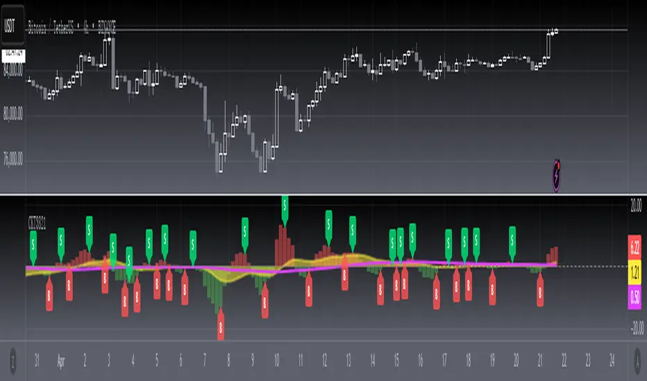
BTCUSDT 1H from TradingView
Tesla 1D from TradingView
American Approximation: Barone-Adesi and Whaley [Loxx]American Approximation: Barone-Adesi and Whaley is an American Options pricing model. This indicator also includes numerical greeks. You can compare the output of the American Approximation to the Black-Scholes-Merton value on the output of the options panel.
An American option can be exercised at any time up to its expiration date. This added freedom complicates the valuation of American options relative to their European counterparts. With a few exceptions, it is not possible to find an exact formula for the value of American options. Several researchers have, however, come up with excellent closed-form approximations. These approximations have become especially popular because they execute quickly on computers compared to numerical techniques. At the end of the chapter, we look at closed-form solutions for perpetual American options.
The Barone-Adesi and Whaley Approximation
The quadratic approximation method by Barone-Adesi and Whaley (1987) can be used to price American call and put options on an underlying asset with cost-of-carry rate b. When b > r, the American call value is equal to the European call value and can then be found by using the generalized Black-Scholes-Merton (BSM) formula. The model is fast and accurate for most practical input values.
American Call
C(S, C, T) = Cbsm(S, X, T) + A2 / (S/S*)^q2 ... when S < S*
C(S, C, T) = S - X ... when S >= S*
where Cbsm(S, X, T) is the general Black-Scholes-Merton call formula, and
A2 = S* / q2 * (1 - e^((b - r) * T)) * N(d1(S*)))
d1(S) = (log(S/X) + (b + v^2/2) * T) / (v * T^0.5)
q2 = (-(N-1) + ((N-1)^2 + 4M/K))^0.5) / 2
M = 2r/v^2
N = 2b/v^2
K = 1 - e^(-r*T)
American Put
P(S, C, T) = Pbsm(S, X, T) + A1 / (S/S**)^q1 ... when S < S**
P(S, C, T) = X - S .... when S >= S**
where Pbsm(S, X, T) is the generalized BSM put option formula, and
A1 = -S** / q1 * (1 - e^((b - r) * T)) * N(-d1(S**)))
q1 = (-(N-1) - ((N-1)^2 + 4M/K))^0.5) / 2
where S* is the critical commodity price for the call option that satisfies
S* - X = c(S*, X, T) + (1 - e^((b - r) * T) * N(d1(S*))) * S* * 1/q2
These equations can be solved by using a Newton-Raphson algorithm. The iterative procedure should continue until the relative absolute error falls within an acceptable tolerance level. See code for details on the Newton-Raphson algorithm.
Inputs
S = Stock price.
K = Strike price of option.
T = Time to expiration in years.
r = Risk-free rate
c = Cost of Carry
V = Variance of the underlying asset price
cnd1(x) = Cumulative Normal Distribution
cbnd3(x) = Cumulative Bivariate Normal Distribution
nd(x) = Standard Normal Density Function
convertingToCCRate(r, cmp) = Rate compounder
Numerical Greeks or Greeks by Finite Difference
Analytical Greeks are the standard approach to estimating Delta, Gamma etc... That is what we typically use when we can derive from closed form solutions. Normally, these are well-defined and available in text books. Previously, we relied on closed form solutions for the call or put formulae differentiated with respect to the Black Scholes parameters. When Greeks formulae are difficult to develop or tease out, we can alternatively employ numerical Greeks - sometimes referred to finite difference approximations. A key advantage of numerical Greeks relates to their estimation independent of deriving mathematical Greeks. This could be important when we examine American options where there may not technically exist an exact closed form solution that is straightforward to work with. (via VinegarHill FinanceLabs)
Things to know
Only works on the daily timeframe and for the current source price.
You can adjust the text size to fit the screen
Generalized Black-Scholes-Merton on Variance Form [Loxx]Generalized Black-Scholes-Merton on Variance Form is an adaptation of the Black-Scholes-Merton Option Pricing Model including Numerical Greeks. The following information is an excerpt from Espen Gaarder Haug's book "Option Pricing Formulas". This version is to price Options using variance instead of volatility.
Black- Scholes- Merton on Variance Form
In some circumstances, it is useful to rewrite the BSM formula using variance as input instead of volatility, V = v^2:
c = S * e^((b - r) * T) * N(d1) - X * e^(-r * T) * N(d2)
p = X * e^(-r * T) * N(-d2) - S * e^((b - r) * T) * N(-d1)
where
d1 = (log(S / X) + (b + V^2 / 2) * T) / (V * T)^0.5
d2 = d1 - (V * T)^0.5
BSM on variance form clearly gives the same price as when written on volatility form. The variance form is used indirectly in terms of its partial derivatives in some stochastic variance models, as well as for hedging of variance swaps. The BSM on variance form moreover admits an interesting symmetry between put and call options as discussed by Adamchuk and Haug (2005) at www.wilmott.com .
c(S, X, T, r, b, V) = -c(-S, -X, -T, -r, -b, -V)
and
p(S, X, T, r, b, V) = -p(-S, -X, -T, -r, -b, -V)
It is possible to find several similar symmetries if we introduce imaginary numbers.
b = r ... gives the Black and Scholes (1973) stock option model.
b = r — q ... gives the Merton (1973) stock option model with continuous dividend yield q.
b = 0 ... gives the Black (1976) futures option model.
b = 0 and r = 0 ... gives the Asay (1982) margined futures option model.
b = r — rf ... gives the Garman and Kohlhagen (1983) currency option model.
Inputs
S = Stock price.
X = Strike price of option.
T = Time to expiration in years.
r = Risk-free rate
cc = Cost of Carry
V = Variance of the underlying asset price
cnd (x) = The cumulative normal distribution function
nd(x) = The standard normal density function
convertingToCCRate(r, cmp ) = Rate compounder
Numerical Greeks or Greeks by Finite Difference
Analytical Greeks are the standard approach to estimating Delta, Gamma etc... That is what we typically use when we can derive from closed form solutions. Normally, these are well-defined and available in text books. Previously, we relied on closed form solutions for the call or put formulae differentiated with respect to the Black Scholes parameters. When Greeks formulae are difficult to develop or tease out, we can alternatively employ numerical Greeks - sometimes referred to finite difference approximations. A key advantage of numerical Greeks relates to their estimation independent of deriving mathematical Greeks. This could be important when we examine American options where there may not technically exist an exact closed form solution that is straightforward to work with. (via VinegarHill FinanceLabs)
Things to know
Only works on the daily timeframe and for the current source price.
You can adjust the text size to fit the screen
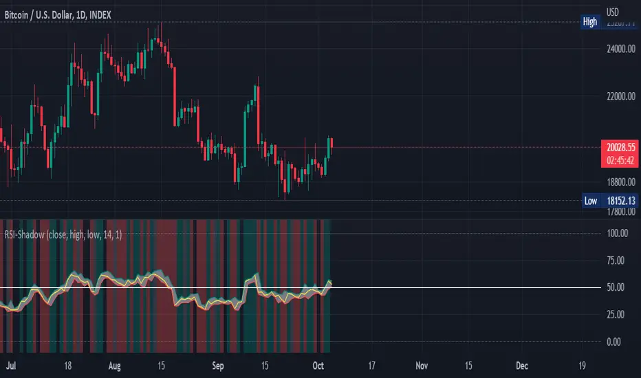
RSI Shadow by TartigradiaHave you ever wondered how much the RSI can vary during an open session? How much wicks can make the RSI overshoots before it retraces for the close?
This indicator plots the RSI shadow, which is the area between the highest and lowest RSI values attained during each open session, from the high/low wick price candle (ie, not the open value).
Technically, we calculate the RSI as usual for all past bars, except for current bar for which we use the high and low values to calculate the RSI Shadow bounds. The invisible PineScript loop then repeats this process for each bar.
In practice, the RSI Shadow provides 2 different informations:
1. This allows to visually represent the variability that historically happened for each bar, which help in better understanding the context at the time and may help predict future similar patterns.
2. The closer the RSI is to one bound, high or low, the more bullish or bearish respectively the price action is. Intuitively, when RSI is close to the high shadow bound, it means that price action is so bullish it often closes in proximity to the highest value attained during the open session, hence very bullish sentiment. And inversely for low and bearish sentiment. To ease visualization of these sentiments, a background highlighting is provided.
The indicator works under all timeframes, but it appears to provide a very reliable information with longer timeframe. The background highlighting showing the bullish/bearish sentiment based on the RSI Shadow appears to indicate crypto market cycles relatively reliably, with 2-3 consecutive bars with the same background color indicating a strong trend.
False positives can be reduced by looking at both the background color and the RSI direction, if both are congruent (ie, both bullish), then the trend indication is good, otherwise the trend indicated by the background color should be disregarded. An option was added to uncolor background if incongruent with RSI's direction.
There is also a "shadow margin" setting that allows to further reduce the number of false positives, at the expense of reduced sensitivity (a margin of 3 seems to eliminate most false positives).
Note: if you need a more complete RSI indicator with overbought/oversold signals, check out RSI+ (alt), which includes all RSI related indicators I make (such as RSI Shadow):
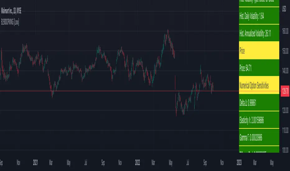
Generalized Black-Scholes-Merton Option Pricing Formula [Loxx]Generalized Black-Scholes-Merton Option Pricing Formula is an adaptation of the Black-Scholes-Merton Option Pricing Model including Numerical Greeks aka "Option Sensitivities" and implied volatility calculations. The following information is an excerpt from Espen Gaarder Haug's book "Option Pricing Formulas".
Black-Scholes-Merton Option Pricing
The BSM formula and its binomial counterpart may easily be the most used "probability model/tool" in everyday use — even if we con- sider all other scientific disciplines. Literally tens of thousands of people, including traders, market makers, and salespeople, use option formulas several times a day. Hardly any other area has seen such dramatic growth as the options and derivatives businesses. In this chapter we look at the various versions of the basic option formula. In 1997 Myron Scholes and Robert Merton were awarded the Nobel Prize (The Bank of Sweden Prize in Economic Sciences in Memory of Alfred Nobel). Unfortunately, Fischer Black died of cancer in 1995 before he also would have received the prize.
It is worth mentioning that it was not the option formula itself that Myron Scholes and Robert Merton were awarded the Nobel Prize for, the formula was actually already invented, but rather for the way they derived it — the replicating portfolio argument, continuous- time dynamic delta hedging, as well as making the formula consistent with the capital asset pricing model (CAPM). The continuous dynamic replication argument is unfortunately far from robust. The popularity among traders for using option formulas heavily relies on hedging options with options and on the top of this dynamic delta hedging, see Higgins (1902), Nelson (1904), Mello and Neuhaus (1998), Derman and Taleb (2005), as well as Haug (2006) for more details on this topic. In any case, this book is about option formulas and not so much about how to derive them.
Provided here are the various versions of the Black-Scholes-Merton formula presented in the literature. All formulas in this section are originally derived based on the underlying asset S follows a geometric Brownian motion
dS = mu * S * dt + v * S * dz
where t is the expected instantaneous rate of return on the underlying asset, a is the instantaneous volatility of the rate of return, and dz is a Wiener process.
The formula derived by Black and Scholes (1973) can be used to value a European option on a stock that does not pay dividends before the option's expiration date. Letting c and p denote the price of European call and put options, respectively, the formula states that
c = S * N(d1) - X * e^(-r * T) * N(d2)
p = X * e^(-r * T) * N(d2) - S * N(d1)
where
d1 = (log(S / X) + (r + v^2 / 2) * T) / (v * T^0.5)
d2 = (log(S / X) + (r - v^2 / 2) * T) / (v * T^0.5) = d1 - v * T^0.5
Inputs
S = Stock price.
X = Strike price of option.
T = Time to expiration in years.
r = Risk-free rate
b = Cost of carry
v = Volatility of the underlying asset price
cnd (x) = The cumulative normal distribution function
nd(x) = The standard normal density function
convertingToCCRate(r, cmp ) = Rate compounder
gImpliedVolatilityNR(string CallPutFlag, float S, float x, float T, float r, float b, float cm, float epsilon) = Implied volatility via Newton Raphson
gBlackScholesImpVolBisection(string CallPutFlag, float S, float x, float T, float r, float b, float cm) = implied volatility via bisection
Implied Volatility: The Bisection Method
The Newton-Raphson method requires knowledge of the partial derivative of the option pricing formula with respect to volatility (vega) when searching for the implied volatility. For some options (exotic and American options in particular), vega is not known analytically. The bisection method is an even simpler method to estimate implied volatility when vega is unknown. The bisection method requires two initial volatility estimates (seed values):
1. A "low" estimate of the implied volatility, al, corresponding to an option value, CL
2. A "high" volatility estimate, aH, corresponding to an option value, CH
The option market price, Cm, lies between CL and cH. The bisection estimate is given as the linear interpolation between the two estimates:
v(i + 1) = v(L) + (c(m) - c(L)) * (v(H) - v(L)) / (c(H) - c(L))
Replace v(L) with v(i + 1) if c(v(i + 1)) < c(m), or else replace v(H) with v(i + 1) if c(v(i + 1)) > c(m) until |c(m) - c(v(i + 1))| <= E, at which point v(i + 1) is the implied volatility and E is the desired degree of accuracy.
Implied Volatility: Newton-Raphson Method
The Newton-Raphson method is an efficient way to find the implied volatility of an option contract. It is nothing more than a simple iteration technique for solving one-dimensional nonlinear equations (any introductory textbook in calculus will offer an intuitive explanation). The method seldom uses more than two to three iterations before it converges to the implied volatility. Let
v(i + 1) = v(i) + (c(v(i)) - c(m)) / (dc / dv(i))
until |c(m) - c(v(i + 1))| <= E at which point v(i + 1) is the implied volatility, E is the desired degree of accuracy, c(m) is the market price of the option, and dc/dv(i) is the vega of the option evaluaated at v(i) (the sensitivity of the option value for a small change in volatility).
Numerical Greeks or Greeks by Finite Difference
Analytical Greeks are the standard approach to estimating Delta, Gamma etc... That is what we typically use when we can derive from closed form solutions. Normally, these are well-defined and available in text books. Previously, we relied on closed form solutions for the call or put formulae differentiated with respect to the Black Scholes parameters. When Greeks formulae are difficult to develop or tease out, we can alternatively employ numerical Greeks - sometimes referred to finite difference approximations. A key advantage of numerical Greeks relates to their estimation independent of deriving mathematical Greeks. This could be important when we examine American options where there may not technically exist an exact closed form solution that is straightforward to work with. (via VinegarHill FinanceLabs)
Things to know
Only works on the daily timeframe and for the current source price.
You can adjust the text size to fit the screen
Sprenkle 1964 Option Pricing Model w/ Num. Greeks [Loxx]Sprenkle 1964 Option Pricing Model w/ Num. Greeks is an adaptation of the Sprenkle 1964 Option Pricing Model in Pine Script. The following information is an except from Espen Gaarder Haug's book "Option Pricing Formulas".
The Sprenkle Model
Sprenkle (1964) assumed the stock price was log-normally distributed and thus that the asset price followed a geometric Brownian motion, just as in the Black and Scholes (1973) analysis. In this way he ruled out the possibility of negative stock prices, consistent with limited liability. Sprenkle moreover allowed for a drift in the asset price, thus allowing positive interest rates and risk aversion (Smith, 1976). Sprenkle assumed today's value was equal to the expected value at maturity.
c = S * e^(rho*T) * N(d1) - (1 - k) * X * N(d2)
d1 = (log(S/X) + (rho + v^2 / 2) * T) / (v * T^0.5)
d2 = d1 - (v * T^0.5)
Inputs
S = Stock price.
X = Strike price of option.
T = Time to expiration in years.
r = Risk-free rate
v = Volatility of the underlying asset price
k = Market risk aversion adjustment
rho = Average growth rate share
cnd (x) = The cumulative normal distribution function
nd(x) = The standard normal density function
nd(x) = The standard normal density function
convertingToCCRate(r, cmp) = Rate compounder
Numerical Greeks or Greeks by Finite Difference
Analytical Greeks are the standard approach to estimating Delta, Gamma etc... That is what we typically use when we can derive from closed form solutions. Normally, these are well-defined and available in text books. Previously, we relied on closed form solutions for the call or put formulae differentiated with respect to the Black Scholes parameters. When Greeks formulae are difficult to develop or tease out, we can alternatively employ numerical Greeks - sometimes referred to finite difference approximations. A key advantage of numerical Greeks relates to their estimation independent of deriving mathematical Greeks. This could be important when we examine American options where there may not technically exist an exact closed form solution that is straightforward to work with. (via VinegarHill FinanceLabs)
Things to know
Only works on the daily timeframe and for the current source price.
You can adjust the text size to fit the screen
Modified Bachelier Option Pricing Model w/ Num. Greeks [Loxx]Modified Bachelier Option Pricing Model w/ Num. Greeks is an adaptation of the Modified Bachelier Option Pricing Model in Pine Script. The following information is an except from Espen Gaarder Haug's book "Option Pricing Formulas".
Before Black Scholes Merton
The curious reader may be asking how people priced options before the BSM breakthrough was published in 1973. This section offers a quick overview of some of the most important precursors to the BSM model. As early as 1900, Louis Bachelier published his now famous work on option pricing. In contrast to Black, Scholes, and Merton, Bachelier assumed a normal distribution for the asset price—in other words, an arithmetic Brownian motion process:
dS = sigma * dz
Where S is the asset price and dz is a Wiener process. This implies a positive probability for observing a negative asset price—a feature that is not popular for stocks and any other asset with limited liability features.
The current call price is the expected price at expiration. This argument yields:
c = (S - X)*N(d1) + v * T^0.5 * n(d1)
and for a put option we get
p = (S - X)*N(-d1) + v * T^0.5 * n(d1)
where
d1 = (S - X) / (v * T^0.5)
Modified Bachelier Model
By using the arguments of BSM but now with arithmetic Brownian motion (normal distributed stock price), we can easily correct the Bachelier model to take into account the time value of money in a risk-neutral world. This yields:
c = S * N(d1) - Xe^-rT * N(d1) + v * T^0.5 * n(d1)
p = Xe^-rT * N(-d1) - S * N(-d1) + v * T^0.5 * n(d1)
d1 = (S - X) / (v * T^0.5)
Inputs
S = Stock price.
X = Strike price of option.
T = Time to expiration in years.
r = Risk-free rate
v = Volatility of the underlying asset price
cnd (x) = The cumulative normal distribution function
nd(x) = The standard normal density function
Numerical Greeks or Greeks by Finite Difference
Analytical Greeks are the standard approach to estimating Delta, Gamma etc... That is what we typically use when we can derive from closed form solutions. Normally, these are well-defined and available in text books. Previously, we relied on closed form solutions for the call or put formulae differentiated with respect to the Black Scholes parameters. When Greeks formulae are difficult to develop or tease out, we can alternatively employ numerical Greeks - sometimes referred to finite difference approximations. A key advantage of numerical Greeks relates to their estimation independent of deriving mathematical Greeks. This could be important when we examine American options where there may not technically exist an exact closed form solution that is straightforward to work with. (via VinegarHill FinanceLabs)
Things to know
Volatility for this model is price, so dollars or whatever currency you're using. Historical volatility is also reported in currency.
There is no dividend adjustment input
Only works on the daily timeframe and for the current source price.

Bachelier 1900 Option Pricing Model w/ Numerical Greeks [Loxx]Bachelier 1900 Option Pricing Model w/ Numerical Greeks is an adaptation of the Bachelier 1900 Option Pricing Model in Pine Script. The following information is an except from Espen Gaarder Haug's book "Option Pricing Formulas"
Before Black Scholes Merton
The curious reader may be asking how people priced options before the BSM breakthrough was published in 1973. This section offers a quick overview of some of the most important precursors to the BSM model. As early as 1900, Louis Bachelier published his now famous work on option pricing. In contrast to Black, Scholes, and Merton, Bachelier assumed a normal distribution for the asset price—in other words, an arithmetic Brownian motion process:
dS = sigma * dz
Where S is the asset price and dz is a Wiener process. This implies a positive probability for observing a negative asset price—a feature that is not popular for stocks and any other asset with limited liability features.
The current call price is the expected price at expiration. This argument yields:
c = (S - X)*N(d1) + v * T^0.5 * n(d1)
and for a put option we get
p = (S - X)*N(-d1) + v * T^0.5 * n(d1)
where
d1 = (S - X) / (v * T^0.5)
Inputs
S = Stock price.
X = Strike price of option.
T = Time to expiration in years.
v = Volatility of the underlying asset price
cnd(x) = The cumulative normal distribution function
nd(x) = The standard normal density function
Numerical Greeks or Greeks by Finite Difference
Analytical Greeks are the standard approach to estimating Delta, Gamma etc... That is what we typically use when we can derive from closed form solutions. Normally, these are well-defined and available in text books. Previously, we relied on closed form solutions for the call or put formulae differentiated with respect to the Black Scholes parameters. When Greeks formulae are difficult to develop or tease out, we can alternatively employ numerical Greeks - sometimes referred to finite difference approximations. A key advantage of numerical Greeks relates to their estimation independent of deriving mathematical Greeks. This could be important when we examine American options where there may not technically exist an exact closed form solution that is straightforward to work with. ( via VinegarHill FinanceLabs )
Things to know
Volatility for this model is price, so dollars or whatever currency you're using. Historical volatility is also reported in currency.
There is no risk-free rate input
There is no dividend adjustment input
Buying & Selling PressureBuying and selling pressure is a volatility indicator which denotes the balance between buyers and sellers inside candlestick.
You set the length to average it just like ATR. But This offers further break down of participants of the market.
Pretty much at any condition of the market the indicator can filter out interesting details to make trading decisions faster or confirm them.
So keep it simple we have two lines
🟢 Green → buying pressure
🔴 Red → selling pressure
If green is rising → Price most likely will grow
If green is rising and red is falling → Price will grow at higher probability
If red is rising → Price most likely will fall
If red is rising and green is falling → Price will fall at higher probability
When they both grow or fall → wait till one of them goes opposite way.
╳ Crossings can indicate turning points for bigger price swings.
Technically by very act of intersecting means that Buying and Selling Pressure are equal.
Can be used for Demand/Supply analysis and evaluate the support/resistance levels.

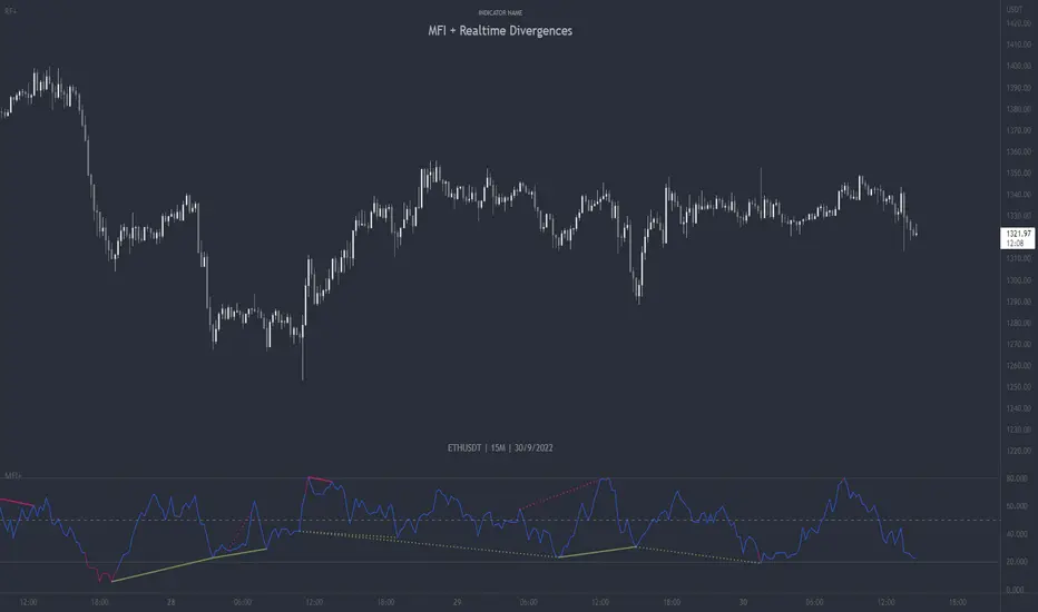
MFI + Realtime DivergencesMoney Flow Index (MFI) + Realtime Divergences + Alerts
This version of the MFI indicator adds the following 5 additional features to the stock MFI:
- Optional divergence lines drawn directly onto the oscillator in realtime.
- Configurable alerts to notify you when divergences occur.
- Configurable lookback periods to fine tune the divergences drawn in order to suit different trading styles and timeframes, including the ability to enable automatic adjustment of pivot period per chart timeframe.
- Background colouring option to indicate when the MFI oscillator has crossed above or below its centerline, or optionally when both the MFI has crossed its centerline and an external oscillator, which can be linked via the settings, has also crossed its centerline.
- Alternate timeframe feature allows you to configure the oscillator to use data from a different timeframe than the chart it is loaded on.
This indicator adds additional features onto the standard MFI , whose core calculations remain unchanged. Namely the configurable option to automatically, quickly and clearly draw divergence lines onto the oscillator for you as they occur in realtime. It also has the addition of unique alerts, so you can be notified when divergences occur without spending all day watching the charts. Furthermore, this version of the TSI comes with configurable lookback periods, which can be configured in order to adjust the sensitivity of the divergences, in order to suit shorter or higher timeframe trading approaches.
What is the Money Flow Index ( MFI )?
Investopedia describes the True Strength Indicator as follows:
“The Money Flow Index ( MFI ) is a technical oscillator that uses price and volume data for identifying overbought or oversold signals in an asset. It can also be used to spot divergences which warn of a trend change in price. The oscillator moves between 0 and 100.
Unlike conventional oscillators such as the Relative Strength Index ( RSI ), the Money Flow Index incorporates both price and volume data, as opposed to just price. For this reason, some analysts call MFI the volume-weighted RSI .”
What are divergences?
Divergence is when the price of an asset is moving in the opposite direction of a technical indicator, such as an oscillator, or is moving contrary to other data. Divergence warns that the current price trend may be weakening, and in some cases may lead to the price changing direction.
There are 4 main types of divergence, which are split into 2 categories;
regular divergences and hidden divergences. Regular divergences indicate possible trend reversals, and hidden divergences indicate possible trend continuation.
Regular bullish divergence: An indication of a potential trend reversal, from the current downtrend, to an uptrend.
Regular bearish divergence: An indication of a potential trend reversal, from the current uptrend, to a downtrend.
Hidden bullish divergence: An indication of a potential uptrend continuation.
Hidden bearish divergence: An indication of a potential downtrend continuation.
Setting alerts.
With this indicator you can set alerts to notify you when any/all of the above types of divergences occur, on any chart timeframe you choose.
Configurable pivot periods.
You can adjust the default pivot periods to suit your prefered trading style and timeframe. If you like to trade a shorter time frame, lowering the default lookback values will make the divergences drawn more sensitive to short term price action.
How do traders use divergences in their trading?
A divergence is considered a leading indicator in technical analysis , meaning it has the ability to indicate a potential price move in the short term future.
Hidden bullish and hidden bearish divergences, which indicate a potential continuation of the current trend are sometimes considered a good place for traders to begin, since trend continuation occurs more frequently than reversals, or trend changes.
When trading regular bullish divergences and regular bearish divergences, which are indications of a trend reversal, the probability of it doing so may increase when these occur at a strong support or resistance level . A common mistake new traders make is to get into a regular divergence trade too early, assuming it will immediately reverse, but these can continue to form for some time before the trend eventually changes, by using forms of support or resistance as an added confluence, such as when price reaches a moving average, the success rate when trading these patterns may increase.
Typically, traders will manually draw lines across the swing highs and swing lows of both the price chart and the oscillator to see whether they appear to present a divergence, this indicator will draw them for you, quickly and clearly, and can notify you when they occur.
Disclaimer: This script includes code from the stock MFI by Tradingview as well as the Divergence for Many Indicators v4 by LonesomeTheBlue.
MTF Stoch RSI + Realtime DivergencesMulti-timeframe Stochastic RSI + Realtime Divergences + Alerts + Pivot lookback periods.
This version of the Stochastic RSI adds the following additional features to the stock UO by Tradingview:
- Optional 3 x Multiple-timeframe overbought and oversold signals, indicating where 3 selected timeframes are all overbought (>80) or all oversold (<20) at the same time, with alert option.
- Optional divergence lines drawn directly onto the oscillator in realtime, with alert options.
- Configurable lookback periods to fine tune the divergences drawn in order to suit different trading styles and timeframes, including the ability to enable automatic adjustment of pivot period per chart timeframe.
- Alternate timeframe feature allows you to configure the oscillator to use data from a different timeframe than the chart it is loaded on.
- Indications where the Stoch RSI is crossing down from above the overbought threshold (<80) and crossing above the oversold threshold (>20) levels on a given user selected timeframe, by printing gold dots on the indicator.
- Also includes standard configurable Stoch RSI options, including k length, d length, RSI length, Stochastic length, and source type (close, hl2, etc)
While this version of the Stochastic RSI has the ability to draw divergences in realtime along with related settings and alerts so you can be notified as divergences occur without spending all day watching the charts, the main purpose of this indicator was to provide the triple multiple-timeframe overbought and oversold confluence signals and alerts, in an attempt to add more confluence, weight and reliability to the single timeframe overbought and oversold states, commonly used for trade entry confluence. It's primary purpose is intended for scalping on lower timeframes, typically between 1-15 minutes. The triple timeframe overbought can often indicate near term reversals to the downside, with the triple timeframe oversold often indicating neartime reversals to the upside. The default timeframes for this confluence are set to check the 1 minute, 5 minute, and 15 minute timeframes, ideal for scalping the < 15 minute charts.
The Stochastic RSI
The popular oscillator has been described as follows:
“The Stochastic RSI is an indicator used in technical analysis that ranges between zero and one (or zero and 100 on some charting platforms) and is created by applying the Stochastic oscillator formula to a set of relative strength index (RSI) values rather than to standard price data. Using RSI values within the Stochastic formula gives traders an idea of whether the current RSI value is overbought or oversold. The Stochastic RSI oscillator was developed to take advantage of both momentum indicators in order to create a more sensitive indicator that is attuned to a specific security's historical performance rather than a generalized analysis of price change.”
How do traders use overbought and oversold levels in their trading?
The oversold level, that is when the Stochastic RSI is above the 80 level is typically interpreted as being 'overbought', and below the 20 level is typically considered 'oversold'. Traders will often use the Stochastic RSI at an overbought level as a confluence for entry into a short position, and the Stochastic RSI at an oversold level as a confluence for an entry into a long position. These levels do not mean that price will necessarily reverse at those levels in a reliable way, however. This is why this version of the Stoch RSI employs the triple timeframe overbought and oversold confluence, in an attempt to add a more confluence and reliability to this usage of the Stoch RSI.
What are divergences?
Divergence is when the price of an asset is moving in the opposite direction of a technical indicator, such as an oscillator, or is moving contrary to other data. Divergence warns that the current price trend may be weakening, and in some cases may lead to the price changing direction.
There are 4 main types of divergence, which are split into 2 categories;
regular divergences and hidden divergences. Regular divergences indicate possible trend reversals, and hidden divergences indicate possible trend continuation.
Regular bullish divergence: An indication of a potential trend reversal, from the current downtrend, to an uptrend.
Regular bearish divergence: An indication of a potential trend reversal, from the current uptrend, to a downtrend.
Hidden bullish divergence: An indication of a potential uptrend continuation.
Hidden bearish divergence: An indication of a potential downtrend continuation.
Setting alerts.
With this indicator you can set alerts to notify you when any/all of the above types of divergences occur, on any chart timeframe you choose, and also when the triple timeframe overbought and oversold confluences occur.
Configurable pivot lookback values.
You can adjust the default pivot lookback values to suit your prefered trading style and timeframe. If you like to trade a shorter time frame, lowering the default lookback values will make the divergences drawn more sensitive to short term price action. By default, this indicator has enabled the automatic adjustment of the pivot periods for 4 configurable timeframes, in a bid to optimise the divergences drawn when the indicator is loaded onto any of the 4 timeframes. These timeframes and the auto adjusted pivot periods on each of them can also be reconfigured within the settings menu.
How do traders use divergences in their trading?
A divergence is considered a leading indicator in technical analysis , meaning it has the ability to indicate a potential price move in the short term future.
Hidden bullish and hidden bearish divergences, which indicate a potential continuation of the current trend are sometimes considered a good place for traders to begin, since trend continuation occurs more frequently than reversals, or trend changes.
When trading regular bullish divergences and regular bearish divergences, which are indications of a trend reversal, the probability of it doing so may increase when these occur at a strong support or resistance level . A common mistake new traders make is to get into a regular divergence trade too early, assuming it will immediately reverse, but these can continue to form for some time before the trend eventually changes, by using forms of support or resistance as an added confluence, such as when price reaches a moving average, the success rate when trading these patterns may increase.
Typically, traders will manually draw lines across the swing highs and swing lows of both the price chart and the oscillator to see whether they appear to present a divergence, this indicator will draw them for you, quickly and clearly, and can notify you when they occur.
Disclaimer: This script includes code from the stock UO by Tradingview as well as the Divergence for Many Indicators v4 by LonesomeTheBlue.

Open High Low StrategyThis is a very simple, yet effective and to some extend widely followed scalping strategy to capture the underling sentiments of the counter whether it will go up or down.
What is it?
This is Open-High-Low (OLH) strategy.
As you already aware of Candlestick patterns, there is patterns called as Marubozu patterns where the sell wick or buy wick either ceases to exists (or very small). This is exactly in the same principle.
In OLH strategy: The buy signal appears when the Open Price is the Low Price. It means if you draw the candlestick, there is no bottom wick. So after the opening of the candle, the demand drives the price up to the level, some selling may or may not come and closes in green. This indicates a strong upward biasness of the underlying counter.
Similarly, a sell signal appears when the Open price is the High Price. It means there is no upper wick. So there is no buying pressure, since the opening of the candle, sellers are in force and pulls down the price to a closing.
This strategy generates the signal at the close of the candle (technically barstate.isconfirmed). Because until the bar is real-time there is no option to know the final closing or high. So you will see the bar on which it generates the buy or sell signal is actually indicates the previous bar as OLH bar.
To determine the Stop-Loss, it uses the most widely known SL calculation of:
For buy signal, it takes the low of the last 7 candles and substract the ATR (Average True Range) of 14-period.
For sell signal, it takes the high of the last 7 candles and add it to the ATR (Average True Range) of 14-period.
One can plot the SL lines as dotted green and red lines as well to see visually.
Default Risk:Reward is 1:2, Can be customizable.
What is Unique?
Of course the utter simplistic nature of this strategy is it's key point. Very easy and intuitive to understand.
There are awesome strategies in this forum that talks about the various indicators combinations and what not.
Instead of all this, in a 15m NSE:NIFTY chart, it generates a good ~ 47% profit-factor with 1:2 Risk Reward ratio. Means if you loose a trade you will loose 1% of account and if you win you will gain 2%. Means 3 trades (2 profits and 1 loss) in a trading session result 3% overall gain for the day. (Assuming you are ready with 1% draw down of your account per trade, at max).
Disclaimer:
This piece of software does not come up with any warrantee or any rights of not changing it over the future course of time.
We are not responsible for any trading/investment decision you are taking out of the outcome of this indicator.

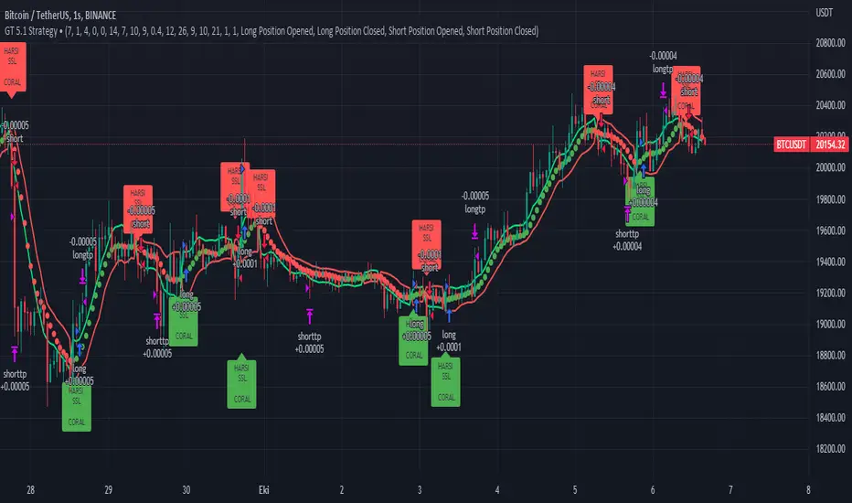
GT 5.1 Strategy═════════════════════════════════════════════════════════════════════════
█ OVERVIEW
People often look an indicator in their technical analysis to enter a position. We may also need to look at the signals of one or more indicators to verify the signals given by some indicators. In this context, I developed a strategy to test whether it really works by choosing some of the indicators that capture trend changes with the same characteristics. Also, since the subject is to catch the trend change, I thought it would be right to include an indicator using the heikin ashi logic. By averaging and smoothing the market noise, Heiken Ashi makes it easier to detect the direction of the trend helps to see possible reversal points on the chart. However, it should be noted that Heiken Ashi is a lagging indicator.
I picked 5 different indicators (but their purpose are similar) and combined them to produce buy and sell signals based on your choice(not repaint). First of all let's get some information about our indicators. So you will understand me why i picked these indicators and what is the meaning of their signals.
1 — Coral Trend Indicator by LazyBear
Coral Trend Indicator is a linear combination of moving averages, all obtained by a triple or higher order exponential smoothing. The indicator comes with a trend indication which is based on the normalized slope of the plot. the usage of this indicator is simple. When the color of the line is green that means the market is in uptrend. But when the color is red that means the market is in downtrend.
As you see the original indicator it is simple to find is it in uptrend or downtrend.
So i added a code to find when the color of the line change. When it turns green to red my script giving sell signals, when it turns red to green it gives buy signals.
I hide the candles to show you more clearly what is happening when you choose only Coral Strategy. But sometimes it is not enough only using itself. Even if green dots turn to red it continues in uptrend. So we need a to look another indicator to approve our signal.
2 — SSL channel by ErwinBeckers
Known as the SSL , the Semaphore Signal Level channel is an indicator that combines moving averages to provide you with a clear visual signal of price movement dynamics. In short, it's designed to show you when a price trend is forming. This indicator creates a band by calculating the high and low values according to the determined period. Simply if you decide 10 as period, it calculates a 10-period moving average on the latest 10 highs. Calculate a 10-period moving average on the latest 10 lows. If the price falls below the low band, the downtrend begins, if the price closes above the high band, the uptrend begins. Lets look the original form of indicator and learn how it using.
If the red line is below and the green band is above, it means that we are in uptrend, and if it is on the opposite side, it means that we are in downtrend. Therefore, it would be logical to enter a position where the trend has changed. So i added a code to find when the crossover has occured.
As you see in my strategy, it gives you signals when the trend has changed. But sometimes it is not enough only using this indicator itself. So lets look 2 indicator together in one chart.
Look circle SSL is saying it is in downtrend but Coral is saying it has entered in uptrend. if we just look to coral signal it can misleads us. So it can be better to look another indicator for validating our signals.
3 — Heikin Ashi RSI Oscillator by JayRogers
The Heikin-Ashi technique is used by technical traders to identify a given trend more easily. Heikin-Ashi has a smoother look because it is essentially taking an average of the movement. There is a tendency with Heikin-Ashi for the candles to stay red during a downtrend and green during an uptrend, whereas normal candlesticks alternate color even if the price is moving dominantly in one direction. This indicator actually recalculates the RSI indicator with the logic of heikin ashi. Due to smoothing, the bars are formed with a slight lag, reflecting the trend rather than the exact price movement. So lets look the original version to understand more clearly. If red bars turn to green bars it means uptrend may begin, if green bars turn to red it means downtrend may begin.
As you see HARSI giving lots of signal some of them is really good but some of them are not very well. Because it gives so much signals Now i will change time period and lets look same chart again.
Now results are better because of heikin ashi's logic. it is not suitable for day traders, it gives more accurate result when using the time period is longer. But it can be useful to use this indicator in short time periods using with other indicators. So you may catch the trend changes more accurately.
4 — MACD DEMA by ToFFF
This indicator uses a double EMA and MACD algorithm to analyze the direction of the trend. Though it might seem a tough task to manage the trades with the help of MACD DEMA once you know how the proper way to interpret the signal lines, it will be an easy task.
This indicator also smoothens the signal lines with the time series algorithm which eventually makes the higher time frame important. So, expecting better results in the lower time frame can result in big losses as the data reading from the MACD DEMA will not be accurate. In order to understand the function of this indicator, you have to know the functions of the EMA also.
The exponential moving average tends to give more priority to the recent price changes. So, expecting better results when the volatility is very high is a very risky approach to trade the market. Moreover, the MACD has some lagging issues compared to the EMA, so it is super important to use a trading method that focuses on the higher time frame only. What does MACD 12 26 Close 9 mean? When the DEMA-9 crosses above the MACD(12,26), this is considered a bearish signal. It means the trend in the stock – its magnitude and/or momentum – is starting to shift course. When the MACD(12,26) crosses above the DEMA-9, this is considered a bullish signal. Lets see this indicator on Chart.
When the blue line crossover red line it is good time to buy. As you see from the chart i put arrows where the crossover are appeared.
When the red line crossover blue line it is good time to sell or exit from position.
5 — WaveTrend Oscillator by LazyBear
This is a technical indicator that creates high and low bands between two values. It then creates a trend indicator that draws waves with highs and lows within these boundaries. WaveTrend is a widely used indicator for finding direction of an asset.
Calculation period: number of candles used to calculate WaveTrend, defaults to 10. Averaging period: number of candles used to average WaveTrend, defaults to 21.
As you see in chart when the lines crossover occured my strategy gives buy or sell signals.
═════════════════════════════════════════════════════════════════════════
█ HOW TO USE
I hope you understand how the indicators I mentioned above work and what they are used for. Now, I will explain in detail how to use the strategy I have created.
When you enter the settings section, you will see 5 types of indicators. If you want to use the signals of the indicators, simply tick the box next to the indicators. Also, under each option there is an area where you can set the "lookback". This setting is a field that will make the signals overlap when you select more than one option. If you are going to trade with only one option, you should make sure that this field is 0. Otherwise, it may continue to generate as many signals as you choose.
Lets see in chart for easy understanding.
As you see chart, if i chose only HARSI with lookback 0 (HARSI and CORAL should be 1 minumum because of algorithm-we looking 1 bar before, others 0 because we are looking crossovers), it will give signals only when harsı bar's color changed. But when i changed Lookback as 7 it will be like this in chart.
Now i will choose 2 indicator with settings of their lookback 0.
As you see it will give signals when both of them occurs same time. But HARSI is an indicator giving very early signal so we can enter position 5-6 bars after the first bar color change. So i will change HARSI Lookback settings as 7. Lets look what happens when we use lookback option.
So it wil be useful to change lookback settings to find best signals in each time period and in each symbol. But it shouldnt be too high. Because you can be late to catch trend's starting.
this is an image of MACD and WAVE trend used and lookback option are both 6.
Now lets see an example with 3 options are chosen with lookback option 11-1-5
Now lets talk about indicators settings. After strategy options you will see each indicators settings, you can change their settings as you desired. So each indicators signal will be changed according to your adjustment.
I left strategy options with default settings. You can change it manually as if you want.
═════════════════════════════════════════════════════════════════════════
█ LIMITATIONS: Don't rely on non-standard charts results. For example Heikin Ashi is a technical analysis method used with the traditional candlestick chart.Heikin Ashi vs. Candlestick Chart: The decisive visual difference between Heikin Ashi and the traditional chart is that Heikin Ashi flattens the traditional candlestick chart using a modified formula.
The primary advantage of Heikin Ashi is that it makes the chart more reader-friendly and helps users identify and analyze trends .
Because Heikin Ashi provides averaged price information rather than real-time price and reacts slowly to volatility — not suitable for scalpers and high-frequency traders. I added HARSI indicator as a supportive signal because it is useful with using CORAL and SSL channel indicators. If you change your candle types to Heikin Ashi , your profit will change in good way but dont rely on it.
═════════════════════════════════════════════════════════════════════════
█ THANKS:
Special thanks to authors of the scripts that i used.
@LazyBear and @ErwinBeckers and @JayRogers and @ToFFF
═════════════════════════════════════════════════════════════════════════
█ DISCLAIMER
Any trade decisions you make are entirely your own responsibility.
Yearly CandlesPlots yearly candles from monthly candles data. This indicator could also be used to view yearly candles of those symbols for which candlesticks are not available in TradingView (for e.g., ECONOMICS:USINTR , ECONOMICS:USIRYY , ECONOMICS:USWG etc)
As these are not out of the box candles they do have these shortcomings -
Last candle's data is not available in status line, a separate label lists OHLC and change details near its close level
The very first candle's width may vary based on how much data is available for that year
Works only with monthly timeframe
Only those indicators that can be added on other indicators can be applied, however, they may still not work as intended as this still technically is a monthly chart!

STD-Adaptive T3 [Loxx]STD-Adaptive T3 is a standard deviation adaptive T3 moving average filter. This indicator acts more like a trend overlay indicator with gradient coloring.
What is the T3 moving average?
Better Moving Averages Tim Tillson
November 1, 1998
Tim Tillson is a software project manager at Hewlett-Packard, with degrees in Mathematics and Computer Science. He has privately traded options and equities for 15 years.
Introduction
"Digital filtering includes the process of smoothing, predicting, differentiating, integrating, separation of signals, and removal of noise from a signal. Thus many people who do such things are actually using digital filters without realizing that they are; being unacquainted with the theory, they neither understand what they have done nor the possibilities of what they might have done."
This quote from R. W. Hamming applies to the vast majority of indicators in technical analysis . Moving averages, be they simple, weighted, or exponential, are lowpass filters; low frequency components in the signal pass through with little attenuation, while high frequencies are severely reduced.
"Oscillator" type indicators (such as MACD , Momentum, Relative Strength Index ) are another type of digital filter called a differentiator.
Tushar Chande has observed that many popular oscillators are highly correlated, which is sensible because they are trying to measure the rate of change of the underlying time series, i.e., are trying to be the first and second derivatives we all learned about in Calculus.
We use moving averages (lowpass filters) in technical analysis to remove the random noise from a time series, to discern the underlying trend or to determine prices at which we will take action. A perfect moving average would have two attributes:
It would be smooth, not sensitive to random noise in the underlying time series. Another way of saying this is that its derivative would not spuriously alternate between positive and negative values.
It would not lag behind the time series it is computed from. Lag, of course, produces late buy or sell signals that kill profits.
The only way one can compute a perfect moving average is to have knowledge of the future, and if we had that, we would buy one lottery ticket a week rather than trade!
Having said this, we can still improve on the conventional simple, weighted, or exponential moving averages. Here's how:
Two Interesting Moving Averages
We will examine two benchmark moving averages based on Linear Regression analysis.
In both cases, a Linear Regression line of length n is fitted to price data.
I call the first moving average ILRS, which stands for Integral of Linear Regression Slope. One simply integrates the slope of a linear regression line as it is successively fitted in a moving window of length n across the data, with the constant of integration being a simple moving average of the first n points. Put another way, the derivative of ILRS is the linear regression slope. Note that ILRS is not the same as a SMA ( simple moving average ) of length n, which is actually the midpoint of the linear regression line as it moves across the data.
We can measure the lag of moving averages with respect to a linear trend by computing how they behave when the input is a line with unit slope. Both SMA (n) and ILRS(n) have lag of n/2, but ILRS is much smoother than SMA .
Our second benchmark moving average is well known, called EPMA or End Point Moving Average. It is the endpoint of the linear regression line of length n as it is fitted across the data. EPMA hugs the data more closely than a simple or exponential moving average of the same length. The price we pay for this is that it is much noisier (less smooth) than ILRS, and it also has the annoying property that it overshoots the data when linear trends are present.
However, EPMA has a lag of 0 with respect to linear input! This makes sense because a linear regression line will fit linear input perfectly, and the endpoint of the LR line will be on the input line.
These two moving averages frame the tradeoffs that we are facing. On one extreme we have ILRS, which is very smooth and has considerable phase lag. EPMA has 0 phase lag, but is too noisy and overshoots. We would like to construct a better moving average which is as smooth as ILRS, but runs closer to where EPMA lies, without the overshoot.
A easy way to attempt this is to split the difference, i.e. use (ILRS(n)+EPMA(n))/2. This will give us a moving average (call it IE /2) which runs in between the two, has phase lag of n/4 but still inherits considerable noise from EPMA. IE /2 is inspirational, however. Can we build something that is comparable, but smoother? Figure 1 shows ILRS, EPMA, and IE /2.
Filter Techniques
Any thoughtful student of filter theory (or resolute experimenter) will have noticed that you can improve the smoothness of a filter by running it through itself multiple times, at the cost of increasing phase lag.
There is a complementary technique (called twicing by J.W. Tukey) which can be used to improve phase lag. If L stands for the operation of running data through a low pass filter, then twicing can be described by:
L' = L(time series) + L(time series - L(time series))
That is, we add a moving average of the difference between the input and the moving average to the moving average. This is algebraically equivalent to:
2L-L(L)
This is the Double Exponential Moving Average or DEMA , popularized by Patrick Mulloy in TASAC (January/February 1994).
In our taxonomy, DEMA has some phase lag (although it exponentially approaches 0) and is somewhat noisy, comparable to IE /2 indicator.
We will use these two techniques to construct our better moving average, after we explore the first one a little more closely.
Fixing Overshoot
An n-day EMA has smoothing constant alpha=2/(n+1) and a lag of (n-1)/2.
Thus EMA (3) has lag 1, and EMA (11) has lag 5. Figure 2 shows that, if I am willing to incur 5 days of lag, I get a smoother moving average if I run EMA (3) through itself 5 times than if I just take EMA (11) once.
This suggests that if EPMA and DEMA have 0 or low lag, why not run fast versions (eg DEMA (3)) through themselves many times to achieve a smooth result? The problem is that multiple runs though these filters increase their tendency to overshoot the data, giving an unusable result. This is because the amplitude response of DEMA and EPMA is greater than 1 at certain frequencies, giving a gain of much greater than 1 at these frequencies when run though themselves multiple times. Figure 3 shows DEMA (7) and EPMA(7) run through themselves 3 times. DEMA^3 has serious overshoot, and EPMA^3 is terrible.
The solution to the overshoot problem is to recall what we are doing with twicing:
DEMA (n) = EMA (n) + EMA (time series - EMA (n))
The second term is adding, in effect, a smooth version of the derivative to the EMA to achieve DEMA . The derivative term determines how hot the moving average's response to linear trends will be. We need to simply turn down the volume to achieve our basic building block:
EMA (n) + EMA (time series - EMA (n))*.7;
This is algebraically the same as:
EMA (n)*1.7-EMA( EMA (n))*.7;
I have chosen .7 as my volume factor, but the general formula (which I call "Generalized Dema") is:
GD (n,v) = EMA (n)*(1+v)-EMA( EMA (n))*v,
Where v ranges between 0 and 1. When v=0, GD is just an EMA , and when v=1, GD is DEMA . In between, GD is a cooler DEMA . By using a value for v less than 1 (I like .7), we cure the multiple DEMA overshoot problem, at the cost of accepting some additional phase delay. Now we can run GD through itself multiple times to define a new, smoother moving average T3 that does not overshoot the data:
T3(n) = GD ( GD ( GD (n)))
In filter theory parlance, T3 is a six-pole non-linear Kalman filter. Kalman filters are ones which use the error (in this case (time series - EMA (n)) to correct themselves. In Technical Analysis , these are called Adaptive Moving Averages; they track the time series more aggressively when it is making large moves.
Included
Bar coloring
Loxx's Expanded Source Types

Softmax Normalized T3 Histogram [Loxx]Softmax Normalized T3 Histogram is a T3 moving average that is morphed into a normalized oscillator from -1 to 1.
What is the Softmax function?
The softmax function, also known as softargmax: or normalized exponential function, converts a vector of K real numbers into a probability distribution of K possible outcomes. It is a generalization of the logistic function to multiple dimensions, and used in multinomial logistic regression. The softmax function is often used as the last activation function of a neural network to normalize the output of a network to a probability distribution over predicted output classes, based on Luce's choice axiom.
What is the T3 moving average?
Better Moving Averages Tim Tillson
November 1, 1998
Tim Tillson is a software project manager at Hewlett-Packard, with degrees in Mathematics and Computer Science. He has privately traded options and equities for 15 years.
Introduction
"Digital filtering includes the process of smoothing, predicting, differentiating, integrating, separation of signals, and removal of noise from a signal. Thus many people who do such things are actually using digital filters without realizing that they are; being unacquainted with the theory, they neither understand what they have done nor the possibilities of what they might have done."
This quote from R. W. Hamming applies to the vast majority of indicators in technical analysis . Moving averages, be they simple, weighted, or exponential, are lowpass filters; low frequency components in the signal pass through with little attenuation, while high frequencies are severely reduced.
"Oscillator" type indicators (such as MACD , Momentum, Relative Strength Index ) are another type of digital filter called a differentiator.
Tushar Chande has observed that many popular oscillators are highly correlated, which is sensible because they are trying to measure the rate of change of the underlying time series, i.e., are trying to be the first and second derivatives we all learned about in Calculus.
We use moving averages (lowpass filters) in technical analysis to remove the random noise from a time series, to discern the underlying trend or to determine prices at which we will take action. A perfect moving average would have two attributes:
It would be smooth, not sensitive to random noise in the underlying time series. Another way of saying this is that its derivative would not spuriously alternate between positive and negative values.
It would not lag behind the time series it is computed from. Lag, of course, produces late buy or sell signals that kill profits.
The only way one can compute a perfect moving average is to have knowledge of the future, and if we had that, we would buy one lottery ticket a week rather than trade!
Having said this, we can still improve on the conventional simple, weighted, or exponential moving averages. Here's how:
Two Interesting Moving Averages
We will examine two benchmark moving averages based on Linear Regression analysis.
In both cases, a Linear Regression line of length n is fitted to price data.
I call the first moving average ILRS, which stands for Integral of Linear Regression Slope. One simply integrates the slope of a linear regression line as it is successively fitted in a moving window of length n across the data, with the constant of integration being a simple moving average of the first n points. Put another way, the derivative of ILRS is the linear regression slope. Note that ILRS is not the same as a SMA ( simple moving average ) of length n, which is actually the midpoint of the linear regression line as it moves across the data.
We can measure the lag of moving averages with respect to a linear trend by computing how they behave when the input is a line with unit slope. Both SMA (n) and ILRS(n) have lag of n/2, but ILRS is much smoother than SMA .
Our second benchmark moving average is well known, called EPMA or End Point Moving Average. It is the endpoint of the linear regression line of length n as it is fitted across the data. EPMA hugs the data more closely than a simple or exponential moving average of the same length. The price we pay for this is that it is much noisier (less smooth) than ILRS, and it also has the annoying property that it overshoots the data when linear trends are present.
However, EPMA has a lag of 0 with respect to linear input! This makes sense because a linear regression line will fit linear input perfectly, and the endpoint of the LR line will be on the input line.
These two moving averages frame the tradeoffs that we are facing. On one extreme we have ILRS, which is very smooth and has considerable phase lag. EPMA has 0 phase lag, but is too noisy and overshoots. We would like to construct a better moving average which is as smooth as ILRS, but runs closer to where EPMA lies, without the overshoot.
A easy way to attempt this is to split the difference, i.e. use (ILRS(n)+EPMA(n))/2. This will give us a moving average (call it IE /2) which runs in between the two, has phase lag of n/4 but still inherits considerable noise from EPMA. IE /2 is inspirational, however. Can we build something that is comparable, but smoother? Figure 1 shows ILRS, EPMA, and IE /2.
Filter Techniques
Any thoughtful student of filter theory (or resolute experimenter) will have noticed that you can improve the smoothness of a filter by running it through itself multiple times, at the cost of increasing phase lag.
There is a complementary technique (called twicing by J.W. Tukey) which can be used to improve phase lag. If L stands for the operation of running data through a low pass filter, then twicing can be described by:
L' = L(time series) + L(time series - L(time series))
That is, we add a moving average of the difference between the input and the moving average to the moving average. This is algebraically equivalent to:
2L-L(L)
This is the Double Exponential Moving Average or DEMA , popularized by Patrick Mulloy in TASAC (January/February 1994).
In our taxonomy, DEMA has some phase lag (although it exponentially approaches 0) and is somewhat noisy, comparable to IE /2 indicator.
We will use these two techniques to construct our better moving average, after we explore the first one a little more closely.
Fixing Overshoot
An n-day EMA has smoothing constant alpha=2/(n+1) and a lag of (n-1)/2.
Thus EMA (3) has lag 1, and EMA (11) has lag 5. Figure 2 shows that, if I am willing to incur 5 days of lag, I get a smoother moving average if I run EMA (3) through itself 5 times than if I just take EMA (11) once.
This suggests that if EPMA and DEMA have 0 or low lag, why not run fast versions (eg DEMA (3)) through themselves many times to achieve a smooth result? The problem is that multiple runs though these filters increase their tendency to overshoot the data, giving an unusable result. This is because the amplitude response of DEMA and EPMA is greater than 1 at certain frequencies, giving a gain of much greater than 1 at these frequencies when run though themselves multiple times. Figure 3 shows DEMA (7) and EPMA(7) run through themselves 3 times. DEMA^3 has serious overshoot, and EPMA^3 is terrible.
The solution to the overshoot problem is to recall what we are doing with twicing:
DEMA (n) = EMA (n) + EMA (time series - EMA (n))
The second term is adding, in effect, a smooth version of the derivative to the EMA to achieve DEMA . The derivative term determines how hot the moving average's response to linear trends will be. We need to simply turn down the volume to achieve our basic building block:
EMA (n) + EMA (time series - EMA (n))*.7;
This is algebraically the same as:
EMA (n)*1.7-EMA( EMA (n))*.7;
I have chosen .7 as my volume factor, but the general formula (which I call "Generalized Dema") is:
GD (n,v) = EMA (n)*(1+v)-EMA( EMA (n))*v,
Where v ranges between 0 and 1. When v=0, GD is just an EMA , and when v=1, GD is DEMA . In between, GD is a cooler DEMA . By using a value for v less than 1 (I like .7), we cure the multiple DEMA overshoot problem, at the cost of accepting some additional phase delay. Now we can run GD through itself multiple times to define a new, smoother moving average T3 that does not overshoot the data:
T3(n) = GD ( GD ( GD (n)))
In filter theory parlance, T3 is a six-pole non-linear Kalman filter. Kalman filters are ones which use the error (in this case (time series - EMA (n)) to correct themselves. In Technical Analysis , these are called Adaptive Moving Averages; they track the time series more aggressively when it is making large moves.
Included:
Bar coloring
Signals
Alerts
Loxx's Expanded Source Types