CyberCandle SwiftEdgeCyberCandle SwiftEdge
Overview
CyberCandle SwiftEdge is a cutting-edge, AI-inspired trading indicator designed for traders seeking precision and clarity in trend-following and swing trading. Powered by SwiftEdge, it combines Heikin Ashi candles, a gradient-colored Exponential Moving Average (EMA), and a Relative Strength Index (RSI) to deliver clear buy and sell signals. Featuring glowing visuals, dynamic signal icons, and a customizable RSI dashboard in the top-right corner, this script offers a futuristic interface for identifying high-probability trade setups on various timeframes (e.g., 1H, 4H).
What It Does
CyberCandle SwiftEdge integrates three powerful components to generate actionable trading signals:
Heikin Ashi Candles: Smooths price action to highlight trends, reducing market noise and making reversals easier to spot.
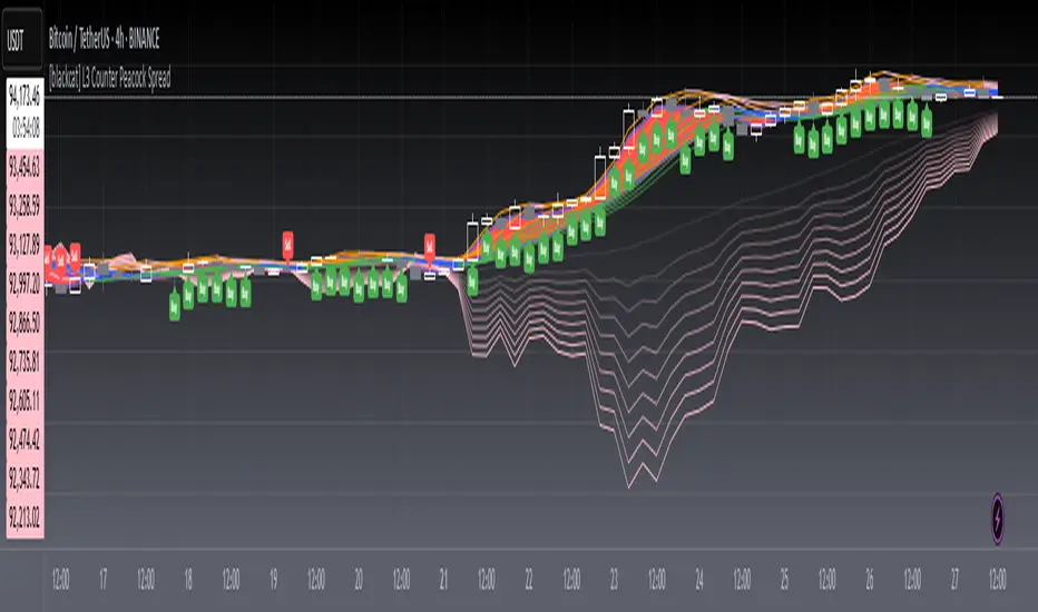
Gradient EMA: A 100-period EMA with dynamic color transitions (blue/cyan for uptrends, red/pink for downtrends) to confirm market direction.
RSI Dashboard: A neon-lit display showing RSI levels, indicating overbought (>70), oversold (<30), or neutral (30-70) conditions.
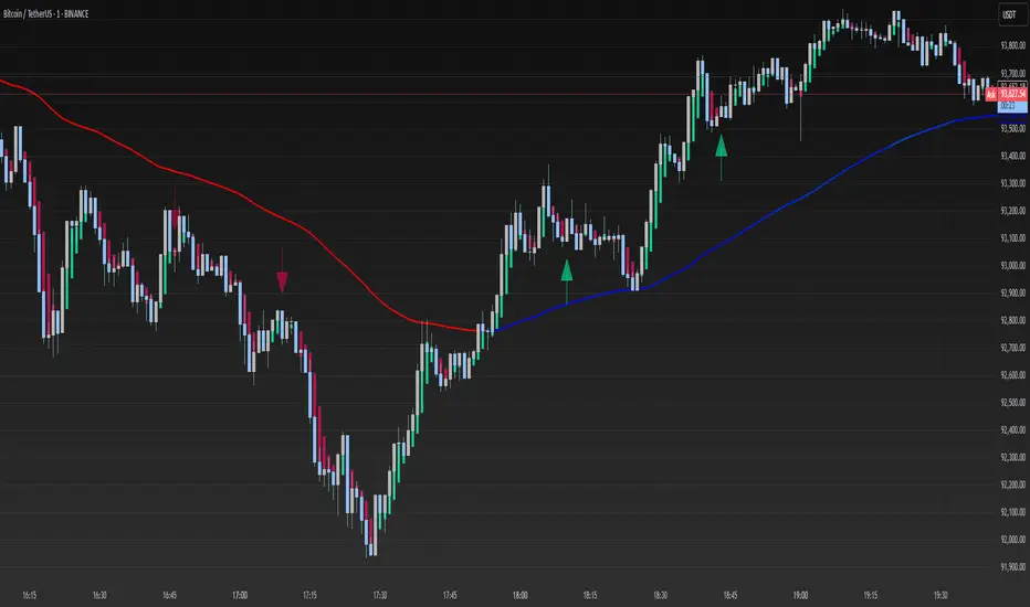
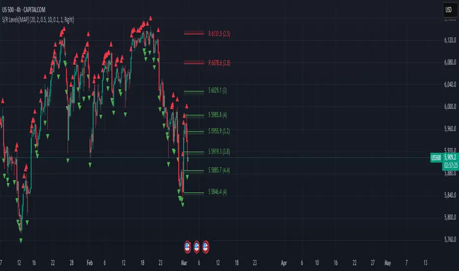
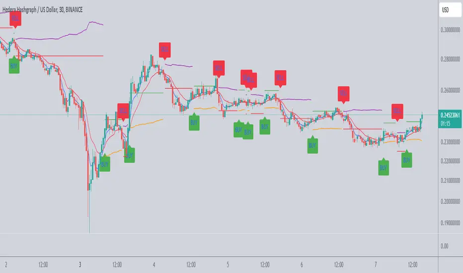
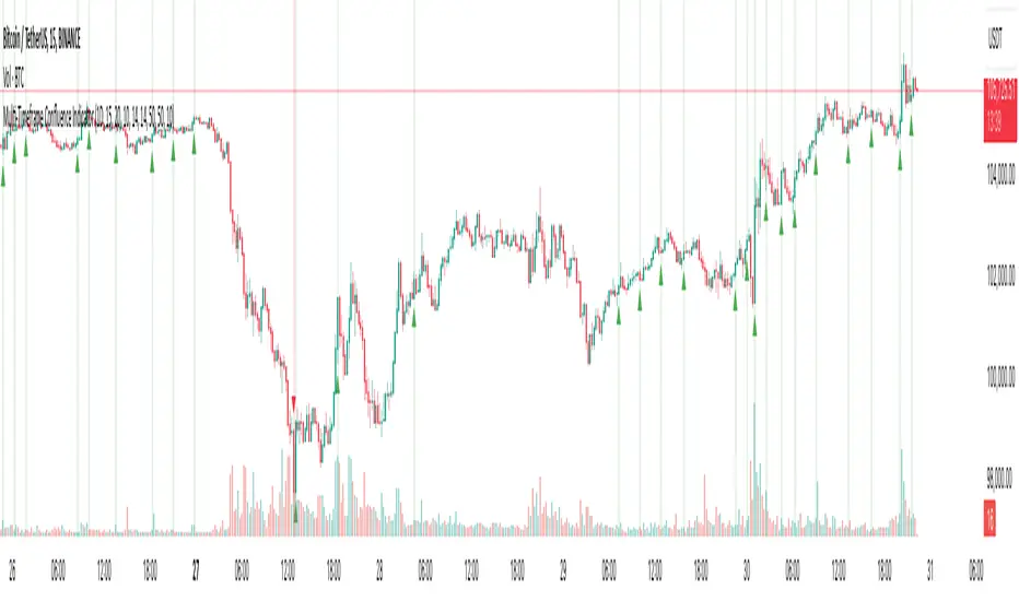
Buy and sell signals are marked with prominent, glowing icons (triangles and arrows) based on trend direction, momentum, and specific Heikin Ashi patterns. The script’s customizable parameters allow traders to tailor the strategy to their preferences, balancing signal frequency and precision.
How It Works
The strategy leverages the synergy of Heikin Ashi, EMA, and RSI to filter trades and highlight opportunities:
Trend Direction: The price must be above the EMA for buy signals (bullish trend) or below for sell signals (bearish trend). The EMA’s gradient color shifts based on its slope, visually reinforcing trend strength.
Momentum Confirmation: RSI must exceed a user-defined threshold (default: 50) for buy signals or fall below it for sell signals, ensuring momentum supports the trade.
Candle Patterns: Buy signals require a green Heikin Ashi candle (close > open), with the two prior candles having minimal upper wicks (≤5% of candle body) and being red (indicating a retracement). Sell signals require a red candle, minimal lower wicks, and two prior green candles.
RSI Dashboard: Positioned in the top-right corner, it features a glowing circle (red for overbought, green for oversold, blue for neutral), the current RSI value, and a status indicator (triangle for extremes, square for neutral). This provides instant momentum insights without cluttering the chart.
By combining Heikin Ashi’s trend clarity, EMA’s directional filter, and RSI’s momentum validation, CyberCandle SwiftEdge minimizes false signals and highlights trades with strong potential. Its vibrant, AI-like visuals make it easy to interpret at a glance.
How to Use It
Add to Chart: In TradingView, search for "CyberCandle SwiftEdge" and add it to your chart. Set the chart to Heikin Ashi candles for optimal compatibility.
Interpret Signals:
Buy Signal: Large green triangles and arrows appear below candles when the price is above the EMA, RSI is above the buy threshold (default: 50), and conditions for a bullish retracement are met. Consider entering a long position with a 1:2 risk/reward ratio.
Sell Signal: Large red triangles and arrows appear above candles when the price is below the EMA, RSI is below the sell threshold (default: 50), and conditions for a bearish retracement are met. Consider entering a short position.
RSI Dashboard: Monitor the top-right dashboard. A red circle (RSI > 70) suggests caution for buys, a green circle (RSI < 30) indicates potential buying opportunities, and a blue circle (RSI 30-70) signals neutrality.
Customize Parameters: Open the indicator’s settings to adjust:
EMA Length (default: 100): Increase (e.g., 200) for longer-term trends or decrease (e.g., 50) for shorter-term sensitivity.
RSI Length (default: 14): Adjust for more (e.g., 7) or less (e.g., 21) responsive momentum signals.
RSI Buy/Sell Thresholds (default: 50): Set higher (e.g., 55) for buys or lower (e.g., 45) for sells to require stronger momentum.
Wick Tolerance (default: 0.05): Increase (e.g., 0.1) to allow larger wicks, generating more signals, or decrease (e.g., 0.02) for stricter conditions.
Require Retracement (default: true): Disable to remove the two-candle retracement requirement, increasing signal frequency.
Trading: Use signals in conjunction with the RSI dashboard and market context. For example, avoid buy signals if the RSI dashboard is red (overbought). Always apply proper risk management, such as setting stop-losses based on recent lows/highs.
What Makes It Original
CyberCandle SwiftEdge stands out due to its futuristic, AI-inspired visual design and user-friendly customization:
Neon Aesthetics: Glowing Heikin Ashi candles, gradient EMA, and dynamic signal icons (triangles and arrows) with RSI-driven transparency create a high-tech, immersive experience.
RSI Dashboard: A compact, top-right display with a neon circle, RSI value, and adaptive status indicator (triangle/square) provides instant momentum insights without cluttering the chart.
Customizability: Users can fine-tune EMA length, RSI parameters, wick tolerance, and retracement requirements via TradingView’s settings, balancing signal frequency and precision.
Integrated Approach: The synergy of Heikin Ashi’s trend clarity, EMA’s directional strength, and RSI’s momentum validation offers a cohesive strategy that reduces false signals.
Why This Combination?
The script combines Heikin Ashi, EMA, and RSI for a complementary effect:
Heikin Ashi smooths price fluctuations, making it ideal for identifying sustained trends and retracements, which are critical for the strategy’s signal logic.
EMA provides a reliable trend filter, ensuring signals align with the broader market direction. Its gradient color enhances visual trend recognition.
RSI adds momentum context, confirming that signals occur during favorable conditions (e.g., RSI > 50 for buys). The dashboard makes RSI intuitive, even for non-technical users.
Together, these components create a balanced system that captures trend reversals after retracements, validated by momentum, with a visually engaging interface that simplifies decision-making.
Tips
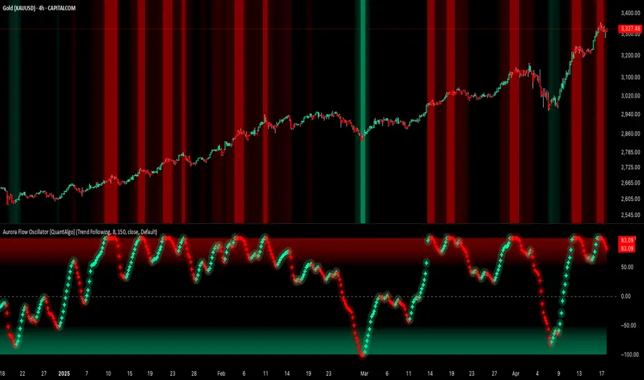
Best used on volatile assets (e.g., BTC/USD, EUR/USD) and higher timeframes (1H, 4H) for clearer trends.
Experiment with parameters in the settings to match your trading style (e.g., increase wick tolerance for more signals).
Combine with other analysis (e.g., support/resistance) for higher-confidence trades.
Note
This indicator is for informational purposes and does not guarantee profits. Always backtest and use proper risk management before trading.
Indicador Pine Script®