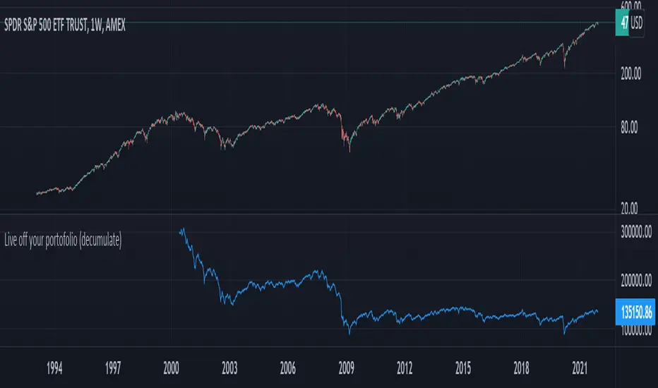
Live off your portofolio (decumulate)This indicator simulates living off your portofolio consisting of a single security or stock such as the SPY etf or even Bitcoin. The simulation starts at a certain point on the chart (which you input as year and month).
Withrawals from the portofolio are made each month according to the yearly withdrawal rate you enter, such as the 4% SWR. The monthly withdrawal income is calculated in USD at the beginning of the retirement period and then adjusted according to the US inflation (CPI) on 01/01 of each year.
The blue graph represents the USD value of the remaining portofolio.
This indicator is meant to be used on daily, weekly or monthly time frame. It may not work properly (and makes little sense to use) on intraday timeframe or larger time frames such as quarterly (3M).
When withdrawing, the indicator considers that fractional stock values can be used (the portofolio value is kept as a float). This may not be true, as most stock brokers currently don't allow this.
It does not explicitly take into account dividends. In order to do this you will have to enable "Adjust for dividends" by clicking on "adj" in the lower right corner of the screen, or by using the indicator on a Total Return (TR) index such as DAX. Unfortunately SPX does not have dividend data, you will have to use the SPY etf (which doesn't have a long history)
Buscar en scripts para "spy"
Random Entries Work!" tHe MaRkEtS aRe RaNdOm ", say moron academics.
The purpose of this study is to show that most markets are NOT random! Most markets show a clear bias where we can make such easy money, that a random number generator can do it.
=== HOW THE INDICATOR WORKS ===
The study will randomly enter the market
The study will randomly exit the market if in a trade
You can choose a Long Only, Short Only, or Bidirectional strategy
=== DEFAULT VALUES AND THEIR LOGIC ===
Percent Chance to Enter Per Bar: 10%
Percent Chance to Exit Per Bar: 3%
Direction: Long Only
Commission: 0
Each bar has a 10% chance to enter the market. Each bar has a 3% to exit the market . It will only enter long.
I included zero commission for simplification. It's a good exercise to include a commission/slippage to see just how much trading fees take from you.
=== TIPS ===
Increasing "Percent Chance to Exit" will shorten the time in a trade. You can see the "Avg # Bars In Trade" go down as you increase. If "Percent Chance to Exit" is too high, the study won't be in the market long enough to catch any movement, possibly exiting on the same bar most of the time.
If you're getting the red screen, that means the strategy lost so much money it went broke. Try reducing the percent equity on the Properties tab.
Switch the start year to avoid/minimize black swan events like the covid drop in 2020.
=== FINDINGS ===
Most markets lose money with a "Random" direction strategy.
Most markets lose ALL money with a "Short Only" strategy.
Most markets make money with a "Long Only" strategy.
Try this strategy on: Bitcoin (BTCUSD) and the NASDAQ (QQQ).
There are two popular memes right now: "Bitcoin to the moon" and "Stocks only go up". Both are seemingly true. Bitcoin was the best performing asset of the 2010's, gaining several billion percent in gains. The stock market is on a 100 year long uptrend. Why? BECAUSE FIAT CURRENCIES ALWAYS GO DOWN! This is inflation. If we measure the market in terms of others assets instead of fiat, the Long Only strategy doesn't work anymore (or works less well).
Try this strategy on: Bitcoin/GLD (BTCUSD/GLD), the Eurodollar (EURUSD), and the S&P 500 measured in gold (SPY/GLD).
Bitcoin measured in gold (BTCUSD/GLD) still works with a Long Only strategy because Bitcoin increased in value over both USD and gold.
The Eurodollar (EURUSD) generally loses money no matter what, especially if you add any commission. This makes sense as they are both fiat currencies with similar inflation schedules.
Gold and the S&P 500 have gained roughly the same amount since ~2000. Some years will show better results for a long strategy, while others will favor a short strategy. Now look at just SPY or GLD (which are both measured in USD by default!) and you'll see the same trend again: a Long Only strategy crushes even when entering and exiting randomly.
=== " JUST TELL ME WHAT TO DO, YOU NERD! " ===
Bulls always win and Bears always lose because fiat currencies go to zero.
You're not underperforming a random number generator, are you?
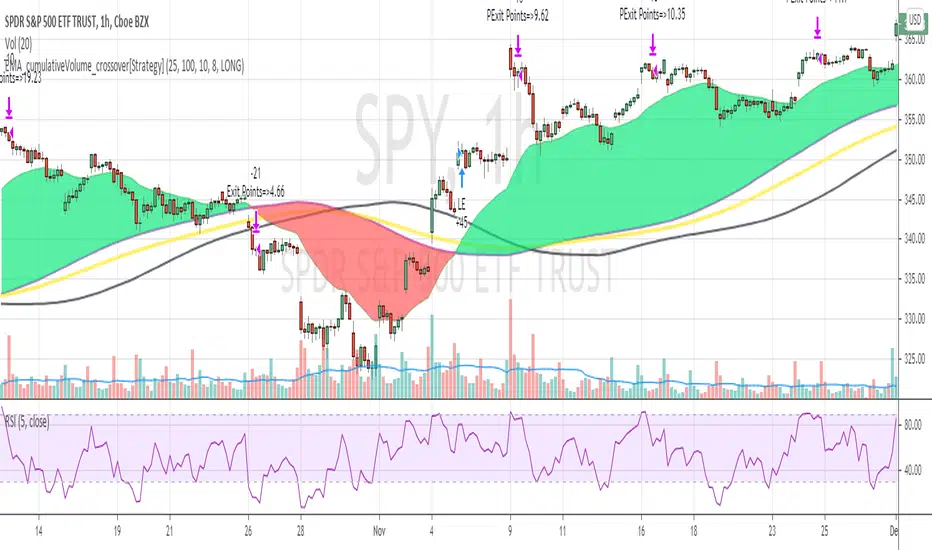
EMA_cumulativeVolume_crossover[Strategy V2]This is variation of EMA_cumulativeVolume_crossover strategy.
instead of cumulative volume crossover, I have added the EMA to cumulative volume of same EMA length.
when EMA crossover EMACumulativeVolume , BUY
when already in LONG position and price crossing over EMACumulativeVolume*2 (orange line in the chart) , Add more
Partial Exit , when RSI 5 crossdown 90
Close All when EMA cross down EMACumulativeVolume
Note
Black Line on the chart is the historical value of EMACumulativeVolume . when EMA area is green and price touch this line closes above it , you can consider consider BUY
I have tested it on SPY , QQQ and UDOW on hourly chart.
EMA setting 25 is working for all of these.
but SPY produces better results on EMA 35 setting
warning
This strategy is published educational purposes only.
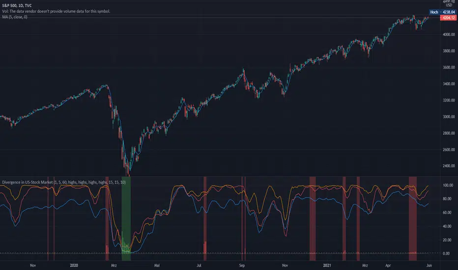
Divergence of Stocks Above MA50 v.s. US-Stock MarketEnglish:
This indicator has been developed as an early warning tool to estimate the probability of correction in the US stock market. It works best in the daily chart.
Function:
1.) "Index-line"
The underlying stock index is converted to a scale between 0% and 100% based on its 52-week highs and lows. Where 100% is closing price at 52-week high and 0% is closing price at 52-week low.
2nd) "Stocks Above MA50".
For each major stock index, there is an index that determines the percentage of stocks above its 50 moving average. For example, for the S&P 500, this is the S5FI.
3) "Divergence
In an efficient market, both lines (index and number of stocks above the 50 MA) would run more or less in sync. A new high in the index would also mean a new high in the stocks trading above the 50 moving average. Often, however, a correction in the index is announced when the number of stocks trading above their 50 MA do not make a new, or even a lower, high while the underlying index marks a new high. The divergence signal measures this divergence of the indices. The higher the bar, the more pronounced the divergence.
How to read the indicator?
If a divergence occurs, then the stops should be tightened. As with any indicator, false signals can occur because a divergence does not automatically lead to a correction. The higher the divergence is indicated, the higher the probability. The strength of a correction cannot be predicted with the indicator.
For which symbols does the indicator work?
The indicator works exclusively for the following symbols:
S&P500: SPX, SPY, ES1!, US500 Index above MA50: S5FI
Russel2000: IWM, US2000, RTY1!, RUT, IWO Index above MA50: R2FI
NASDAQ100: NDX, NAS100, NQ1!, US100, QQQ Index above MA50: NDFI
NASDAQ: IXIC, ONEQ, QCN1!, NDAQ Index above MA50: NCFI
NYSE: XAX, NYA Index above MA50: MMFI
DowJones100: DJX, DJI, DIA, MYM1!, YM1! Index above MA50: DIFI
DowJonesComp: DOW, IYY Index above MA50: DCFI
Deutsch:
Dieser Indikator ist als Frühwarninstrument zur Einschätzung der Korrekturwahrscheinlichkeit im US-Aktienmarkt entwickelt worden. Er funktioniert am besten im Tages-Chart.
Funktion:
1.) „Index-line“
Der zugrunde liegende Aktienindex wird bezogen auf seine 52Wochen Hochs und Tiefs in eine Skala zwischen 0% und 100% umgerechnet. Dabei sind 100% Schlusskurs auf 52-Wochen Hoch und 0% Schlusskurs auf 52-Wochen Tief.
2.) „Stocks Above MA50“
Zu jedem Hauptaktienindex gibt es einen Index, der den Prozentwert der Aktien über Ihrem 50 gleitenden Durchschnitt ermittelt. Beim S&P 500 ist das z.B. der S5FI.
3.) „Divergence“
In einem effizienten Markt würden beide Linien (Index und Anzahl Aktien über dem 50 MA) mehr oder weniger synchron laufen. Ein neues Hoch im Index würde auch ein neues Hoch bei den Aktien, die über dem 50 gleitenden Durchschnitt notieren, bedeuten. Oft jedoch kündigt sich eine Korrektur im Index an, wenn die Anzahl der Aktien, die über ihrem 50 MA notieren kein neues, oder sogar ein niedrigeres Hoch machen, während der zu Grunde liegende Index ein neues Hoch markiert. Das Divergenz-Signal misst diese auseinanderlaufen der Indices. Je höher der Balken, umso stärker ist die Divergenz ausgeprägt.
Wie ist der Indikator zu lesen?
Wenn eine Divergenz auftritt, dann sollten die Stopps enger herangezogen werden. Es kann wie bei jedem Indikator zu Fehlsignalen kommen, da eine Divergenz nicht automatisch zu einer Korrektur führen muss. Die Wahrscheinlichkeit ist um so höher, je höher die Divergenz angezeigt wird. Die Stärke einer Korrektur kann mit dem Indikator nicht prognostiziert werden.
Für welche Symbole funktioniert der Indikator?
Der Indikator funktioniert ausschließlich für folgende Symbole:
S&P500: SPX, SPY, ES1!, US500 Index über MA50: S5FI
Russel2000: IWM, US2000, RTY1!, RUT, IWO Index über MA50: R2FI
NASDAQ100: NDX, NAS100, NQ1!, US100, QQQ Index über MA50: NDFI
NASDAQ: IXIC, ONEQ, QCN1!, NDAQ Index über MA50: NCFI
NYSE: XAX, NYA Index über MA50: MMFI
DowJones100: DJX, DJI, DIA, MYM1!, YM1! Index über MA50: DIFI
DowJonesComp: DOW, IYY Index über MA50: DCFI
Indices trendsAccording to the Dow theory, indices must confirm each other. Based on this idea, I develop an indices trends indicator, including SPY, DIA, and QQQ. The indices trends were calculated based on the average of the short- (blue) and intermediate-term (orange) changes of indices moving average slopes. In addition, IWM trends are shown as a reference in gray color.
Use this indicator together with one of SPY, DIA, QQQ, or IWM to show the overall market conditions.

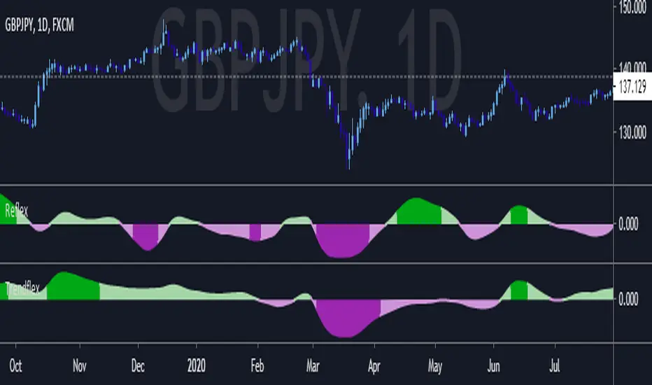
Trendflex - Another new Ehlers indicatorSource: Stocks and Commodities V38
Hooray! Another new John Ehlers indicator!
John claims this indicator is lag-less and uses the SPY on the Daily as an example.
This indicator is a slight modification of Reflex, which I have posted here
I think it's better for Stocks and ETFs than Reflex since it factors in long trends. It tends to keep you in winning trades for a long time.
I believe this indicator can be used for entries or exits, potentially both.
Entry
1. Entering Long positions at the pivot low points (Stocks and ETFs)
2. Entering Long when the Reflex crosses above the zero lines (Stocks, ETFs, Commodities )
Exit
1. Exiting Long positions at a new pivot high point (Stocks and ETFs)
2. Exiting Long when the Reflex crosses below the zero lines (Stocks, ETFs, Commodities )
In this example, I place a Long order on the SPY every time the Reflex crosses above the zero level and exit when it crosses below or pops my stop loss, set at 1.5 * Daily ATR.
2/3 Wins
+16.05%
Let me know in the comment section if you're able to use this in a strategy.

Reflex - A new Ehlers indicatorSource: Stocks and Commodities V38
Hooray! A new John Ehlers indicator!
John claims this indicator is lag-less and uses the SPY on the Daily as an example.
He states that drawing a line from peak to peak (or trough to trough) will correspond perfectly with the Asset.
I have to say I agree! There is typically one bar of lag or no lag at all!
I believe this indicator can be used for either entries or exits, but not both.
Entry
1. Entering Long positions at the pivot low points (Stocks and ETFs)
2. Entering Long when the Reflex crosses above the zero lines (Stocks, ETFs, Commodities)
Exit
1. Exiting Long positions at a new pivot high point (Stocks and ETFs)
2. Exiting Long when the Reflex crosses below the zero lines (Stocks, ETFs, Commodities)
In this example, I place a Long order on the SPY every time the Reflex crosses above the zero level and exit when it crosses below or pops my stop loss, set at 1.5 * Daily ATR.
4/6 Wins
+10.76%
For me, that's good enough to create a strategy and backtest on several Indices and ETFs, which is what I have a hunch this will work on.
I think there is a lot of promise from a single Indicator!
Let me know in the comment section if you're able to use this in a strategy.
Hide Extended Hours/non-intraday American BarsOnly works with American bar style.
Not works with Candles.
--------
This script can hide the extended hours/non-intraday bars and leave the intraday bars only, especially for future users, such as ES/NQ/RTY/YM, etc.,.
Now you can find the intraday support/resistance quite easily!
Example, as a ES investor, you can easily find the intraday support/resistance level ,which is almost equal to SPY / SPX , no longer need to check SPY / SPX separately again, saving your time a lot.
--------
IMPORTANT INSTRUCTION
In order to make the script work, you have to bring it to the most top visual layer.
Please do as the following steps:
Add the script to chart
Hover mouse on the script name, and tap the right-most 'more' button (which appears as 3 dots)
Select "Visual Order", then select "Bring to front".
Done!
Also, in order to have a better view effect and make the bars COMPLETELY "Hidden", you can adjust the hidden bar color in the "setting" menu to the exact color of your chart background.

Swing-Trade-Stocks SystemThis is a simple swing trade system inspired by sources on the internet. The rules are as follows:
Buy when first green arrow appears after 10ma above 30ma
Set stop-loss below most recent support
Set take-profit below most recent swing point high or wait until price closes below 30ma (red)
Short when first purple arrow appears after 10ma below 30ma
Set stop-loss above most recent resistance
Set take-profit above most recent swing point low or wait until price closes above 30ma (red)
The background color changes based on the direction of SPY. If SPY is going down (10ma < 30ma) the
background will be red and only short indicators (purple arrows) will appear. If SPY is going up (10ma > 30ma),
the background will be green and only long indicators (green arrows) will appear.
Happy trading!
Market Internals [Makit0] MARKET INTERNALS INDICATOR v0.5beta
Market Internals are suitable for day trade equity indices, named SPY or /ES, please do your own research about what they are and how to use them
This scripts plots the NYSE market internals charts as an indicator for an easy and full visualization of market internal structure all in one chart, useful for SPY and /ES trading
Description of the Market Internals
- TICK: NYSE stocks ticking up vs stocks ticking down, extreme values may point to trend continuation on trending days or reversal in non trending days, example of extreme values can be 800 and 1000
- ADD: NYSE stocks going up vs stocks going down, if price auctions around the zero line may be a non trend day, otherwise may be a trend day
- VOLD: NYSE volume of stocks up vs volume of stocks going down, identify clearly where the volume is going, as example if volume is flowing down may be a good idea no to place longs
- TRIN: NYSE up stocks vs down stocks ratio divided by up volume vs down volume ratio. A value of 1 indicates parity, below that the strength is on the long side, above the strength is in the short side.
A basic use of market internals may be looking for divergences, for example:
- /ES is trading in a range but ADD and VOLD are trending up nonstop, may /ES will break the range to the upside
- /ES is trading in a range and ADD and VOLD are trading around the zero line but got an extreme reading on TICK, may be a non trending day and the TICK extreme reading is at one of the extremes of the /ES range, may be a good probability trade to fade that move
- /ES is trading in a trend to the downside, ADD and VOLD too, you catch a good portion of the move but are fearful to flat and miss more gains, you see in the TICK a lot of extreme values below -800 so your're confident in the continuation of the downtrend, until the TICK goes beyond -1000 and you use that signal to go flat
Market internals give you context and confirmation, price in /ES may be trending but if market internals do not confirm the move may a reversal is on its way
Price is an advertise, you can see the real move in the structure below, in the behavior of the individual components of the market, those are the real questions:
- How many stocks are going up/down (ADD)
- How many volume is flowing up/down (VOLD)
- How many stocks are ticking up/down (TICK)
- What is the overall volume breath of the market (TRIN)
FEATURES:
- Plot one of the four basic market internal indices: TICK, ADD, VOLD and TRIN
- Show labels with values beyond an user defined threshold
- Show ZERO line
- Show user defined Dotted and Dashed lines
- Show user defined moving average
SETTINGS:
- Market internal: ticker to plot in the indicator, four options to choose from (TICK, ADD, VOLD and TRIN)
- Labels threshold: all values beyond this will be ploted as labels
- Dot lines at: two dotted lines will be plotted at this value above and below the zero line
- Dash lines at: two dashed lines will be plotted at this value above and below the zero line
- MA type: two options avaiable SMA (Simple Moving Average) or EMA (Exponential Moving Average)
- MA length: number of bars to calculate the moving average
- Show zero line: show or hide zero line
- Show dot line: show or hide dotted lines
- Show dash line: show or hide dashed lines
- Show labels: show or hide labels
GOOD LUCK AND HAPPY TRADING

Hide extended hours/non-intraday barsEspecially for future users, such as ES/NQ/RTY/YM, etc., this script can hide the extended hours/non-intraday bars and leave the intraday bars only.
With this script , you can find the intraday support/resistance quite easily!
Example, if you are a ES investor, you can easily find the intraday support/resistance level ,which is almost equal to SPY, with this script, and no need to check SPY separately again , saving your time a lot.
Note: Please couple this script with American Bars. If you use candle charts, the upper/lower pins of the candle can't be hidden with the bars together, which is restricted by the code editor itself...
Kozlod - RSI Strategy - 1 minuteStarted to play with very simple strategies. Trying to find ones with optimal parameters which work well for certain symbols/timeframe.
Found that basic RSI strategy without any position management with high RSI length (65 in this script) works pretty good for 1m chart for few stocks.
It's also not bad for AAPL , SPY .
It might not work very good on it's not but can give you a pretty good base for more complicated indicators.
And remember:
Past performance does not guarantee future results.

Willams %RwEMAspy
Was looking for something else when surfed into an old question
wanting %R 21 period with EMA 13 period of the %R signal
and being a rookie at this, made this code to post for them.
Tried to comment the script in such a way that other rookies
like me could make better sense of what is being done. Hope
this helps someone. I find it useful as one of my indicators for
trading.
Pinescript for tradingview.com user Tom1trader
All time frames.
Interpretation:
%R (Red) crosses above it's average (Blue) - bull
%R crosses below it's average - bear. Background
color changes green-up red-down with above crossings.
Most but not all of serious price movement takes place
from the time the %R (red) goes into oversold (or bought) and
exits again.
%R centerline crosses can also be useful.
I use various indicators and want all of the confirmation
that I can get for expectations BUT I never know what the
next bar will do and define my risks accordingly.
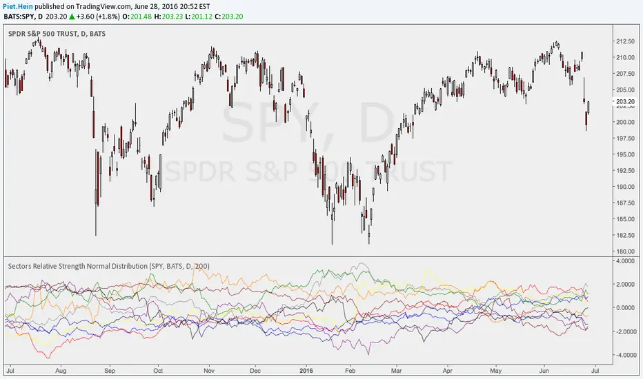
Sectors Relative Strength Normal DistributionI wrote this indicator as an attempt to see the Relative Strengths of different sectors in the same scale, but there is also other ways to do that.
This indicator plots the normal distribution for the 10 sectors of the SPY for the last X bars of the selected resolution, based on the selected comparative security. It shows which sectors are outperforming and underperforming the SPY (or any other security) relatively to each other by the given deviation.
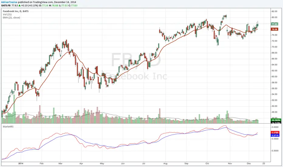
MarketRSThe strength of a stock relative to the market (SPY) is an import indicator accumulation of a stock by institutionan funds, especially during a market decline. This indicator plot the ratio of a security/SPY and plots a fast (5 period) and slow (21 period) EMA.
Iron Fly SPX 0DTE Strategy🦋 Iron Fly 0DTE Strategy
A simple indicator that tells you when to open and close Iron Fly options trades on SPX. Get alerts, execute manually in your broker.
What Does This Do?
This indicator watches the market and sends you alerts:
"OPEN" alert = Good time to sell an Iron Fly at this strike
"CLOSE" alert = Time to close your position (take profit or cut loss)
"EXPIRED" alert = End of day, let it expire or close manually
You receive the exact strikes to trade. You execute in your broker.
What is an Iron Fly?
An Iron Fly is a bet that the price stays near a certain level until end of day.
You collect money upfront (premium). If price stays close to your strike, you keep most of it. If price moves too far, you lose money (but your loss is capped).
The Trade (4 legs):
SELL a Call at the strike (collect premium)
SELL a Put at the strike (collect premium)
BUY a Call above for protection (costs premium)
BUY a Put below for protection (costs premium)
Net result: You collect premium. Max profit if price closes exactly at strike. Max loss is limited by your protective wings.
For a detailed explanation with visuals, read: kriyafx.substack.com
How to Use
Step 1: Add to Chart
Add indicator to SPX or SPY chart (1-5 minute timeframe recommended)
Step 2: Set Up Alerts
Create alert: Condition = "Iron Fly 0DTE" → "Any alert() function call"
Step 3: Wait for OPEN Alert
When you get an alert like this:
🦋 OPEN IRON FLY
Strike: 6980
Wings: ±30 pts
Sell 6980 Call
Sell 6980 Put
Buy 7010 Call
Buy 6950 Put
Step 4: Execute in Your Broker
Open your options broker, find today's expiration (0DTE), and enter the 4-leg trade at the strikes shown. Check the premium you'll collect - make sure it's worth the risk.
Step 5: Wait for CLOSE Alert
The indicator monitors your position. When it's time to exit, you get:
🦋 CLOSE IRON FLY
Strike: 6980
Reason: Price moved up past exit threshold
Buy to Close 6980 Call
Buy to Close 6980 Put
Sell to Close 7010 Call
Sell to Close 6950 Put
Close your position in your broker.
The Status Panel
The box on your chart shows:
Positions - How many flies are currently open
Market - Is it a good time to trade? (GOOD/OK/RISKY/STOP)
Wings - Current suggested wing width
Exit @ - How far price can move before you should exit
Trades - How many trades today vs your daily limit
Settings Explained
Entry Aggressiveness
How often should new trades open?
LOW = Fewer trades, more selective (beginner friendly)
MID = Balanced (recommended)
HIGH = More trades, more active (experienced)
Exit Aggressiveness
How long to hold before exiting?
LOW = Exit early, smaller wins, protected (beginner friendly)
MID = Balanced hold time (recommended)
HIGH = Hold longer, bigger potential wins but more risk
Max Concurrent Flies
How many positions open at the same time? Start with 1-2.
Max Trades Per Day
Daily limit to prevent overtrading. Start with 5-10.
When Does It Work Best?
Sideways, choppy markets (price not trending hard)
Normal volatility days (not FOMC, CPI, or earnings)
US market hours (10 AM - 4 PM Eastern)
When Does It NOT Work?
Strong trending days (price keeps going one direction)
High volatility events (news releases)
When the indicator shows RISKY or STOP
Important: Check Your Premium!
The indicator tells you WHEN to trade and at WHAT strikes. It does NOT tell you the price.
Before entering any trade:
Check the premium in your broker
Make sure the credit received is worth the max loss risk
Consider bid-ask spreads (wider = harder to profit)
If the premium looks bad, skip the trade
Start Small
Paper trade first to understand the signals
Start with 1 fly at a time
Use Entry LOW + Exit LOW when learning
Only risk money you can afford to lose
Risk Warning
Options trading is risky. Iron Flies can lose money - your max loss is the wing width minus premium collected. This indicator gives signals, not guarantees.
This is educational, not financial advice
Past signals don't guarantee future results
You can lose your entire premium
Always know your max loss before entering
Learn More
Full strategy explanation with charts and examples:
kriyafx.substack.com

ORB + Expected Move + Trade Bias RWCORB + Expected Move + Trade Bias v3
Overview
A comprehensive 0DTE SPX options trading indicator designed to identify optimal credit spread and iron condor setups based on Opening Range Breakout (ORB) analysis, Expected Move calculations, VWAP dynamics, and multi-factor confidence scoring. The indicator provides specific strike suggestions, real-time position management signals, and exit warnings.
Who This Is For
This indicator is built for traders who sell 0DTE SPX credit spreads (put spreads, call spreads, or iron condors) and want a systematic, data-driven approach to:
Determine trade direction (bullish, bearish, or neutral)
Select appropriate strikes based on market conditions
Manage positions with clear exit signals
Core Components
1. Opening Range Breakout (ORB)
The ORB establishes the initial trading range after market open, serving as the foundation for trade bias determination.
Settings:
ORB Period: Choose 15, 30, 45, or 60 minutes
Shorter periods (15-30 min) = more signals, more noise
Longer periods (45-60 min) = fewer signals, more reliable ranges
ORB Breakout Buffer %: Percentage buffer beyond ORB high/low before confirming breakout (default 0.1%)
Colors: Customize ORB high (green), low (red), and fill colors
How It Works:
Tracks the high and low during the ORB period
After ORB completes, monitors for breakouts above/below with buffer
Counts consecutive bars above/below ORB for confirmation
2. Expected Move (EM)
Calculates the statistically expected daily range based on Average True Range (ATR).
Settings:
ATR Length: Lookback period for ATR calculation (default 14)
ATR Multiplier: Scale the expected move (default 1.0)
Colors: Customize expected move lines and fill
How It Works:
Pulls daily ATR from the previous session
Projects expected move boundaries from session open
Used for strike distance calculations and range containment analysis
3. VWAP Analysis
Volume Weighted Average Price with standard deviation bands provides trend confirmation and stretch detection.
Settings:
Show VWAP: Toggle VWAP line visibility
Show VWAP StdDev Bands: Toggle ±1 standard deviation bands
VWAP Band Multiplier: Adjust band width (default 1.0)
VWAP Slope Lookback: Bars to measure VWAP slope (default 10)
Key Metrics:
VWAP Slope: Normalized slope indicating trend strength
Strong Up (↑↑): > 0.5
Up (↑): 0.3 to 0.5
Flat (—): -0.3 to 0.3
Down (↓): -0.5 to -0.3
Strong Down (↓↓): < -0.5
Stretched Detection: Warns when price is >1.5 standard deviations from VWAP
4. Prior Day Levels (PDH/PDL)
Yesterday's high and low serve as key support/resistance levels where institutional orders often cluster.
Settings:
Show Prior Day High/Low: Toggle PDH/PDL lines
Show Prior Day Close: Optional PDC line
Colors: Customize PDH (teal), PDL (orange), PDC (gray)
Why It Matters:
Price above PDH = strong bullish continuation signal
Price below PDL = strong bearish continuation signal
Price between PDH/PDL = range-bound, favors iron condors
Strikes are adjusted to respect these levels as potential support/resistance
Trade Signal System
Signal Time
Settings:
Signal Time (ET): Choose when the indicator evaluates and locks in the trade signal
1100 = 8:00 AM PT / 11:00 AM ET
1115 = 8:15 AM PT / 11:15 AM ET (default)
1130 = 8:30 AM PT / 11:30 AM ET
1145 = 8:45 AM PT / 11:45 AM ET
1200 = 9:00 AM PT / 12:00 PM ET
Recommendation: Later signal times (8:30-9:00 AM PT) provide more data and reduce morning fakeout signals, but leave less time for theta decay.
Confidence Scoring (9 Factors)
The indicator calculates three scores: Iron Condor (IC), Bullish, and Bearish. The highest score determines the signal.
Factor 1: Price Position vs ORB (max 40 pts)
Inside ORB → +35-40 IC points
Above ORB (confirmed breakout) → +40 Bull points
Below ORB (confirmed breakout) → +40 Bear points
Factor 2: VWAP Slope (max 30 pts)
Flat slope → +25 IC points
Strong positive slope → +30 Bull points
Strong negative slope → +30 Bear points
Factor 3: Price vs VWAP Position (max 20 pts)
Above upper band → +20 Bull points
Below lower band → +20 Bear points
Near VWAP → +12 IC points
Factor 4: VWAP Consistency (max 15 pts)
70%+ bars above VWAP → +15 Bull points
70%+ bars below VWAP → +15 Bear points
Mixed → +10 IC points
Factor 5: Move from Open (max 20 pts)
30% of EM up → +20 Bull points
30% of EM down → +20 Bear points
<12% move either way → +15 IC points
Factor 6: Trend Structure (max 15 pts)
Higher highs + higher lows → +15 Bull points
Lower lows + lower highs → +15 Bear points
No clear structure → +8 IC points
Factor 7: Day Range Containment (max 15 pts)
Range <35% of EM → +15 IC points
Range <50% of EM → +8 IC points
Range >65% of EM → Points to directional score
Factor 8: Gap Behavior (max 12 pts)
Gap up, unfilled, above ORB → +12 Bull points
Gap down, unfilled, below ORB → +12 Bear points
Gap filled, inside ORB → +8 IC points
Factor 9: Prior Day High/Low (max 20 pts)
Above PDH → +20 Bull points
Below PDL → +20 Bear points
Between PDH/PDL → +15-20 IC points
Alignment Bonuses (max 25 pts)
Additional points when multiple factors align in the same direction.
Signal Types
SignalMeaningTradeIRON CONDORRange-bound conditionsSell both put and call credit spreadsPUT SPREADBullish conditionsSell put credit spread onlyCALL SPREADBearish conditionsSell call credit spread onlyNO TRADEConflicting signals or low confidenceStay out
Confidence Levels
ConfidenceColorStrike Mode75%+Green🍆 AGGRESSIVE (tighter strikes, more premium)60-75%Lime/Yellow🌶️ NORMAL (balanced strikes)45-60%Yellow/Orange🐢 CONSERVATIVE (wider strikes, safer)<45%Orange/RedNO TRADE triggered
Strike Suggestions
Base Calculation
For Iron Condors: Strikes are calculated from current price at signal time as the midpoint, ensuring symmetric risk on both sides.
For Directional Spreads: Strikes are calculated from session open, betting on continuation.
Put Strike = Midpoint - (Expected Move × Distance)
Call Strike = Midpoint + (Expected Move × Distance)
Distance Settings:
High Confidence (75%+): 0.60 EM (default) - Tighter strikes, more premium
Mid Confidence (60-75%): 0.70 EM (default) - Balanced
Low Confidence (<60%): 0.80 EM (default) - Wider strikes, safer
Skew Adjustments
When Auto-Adjust for Skew is enabled, strikes are asymmetrically adjusted based on:
VIX Level:
VIX > 20: Puts pushed wider (-0.05), Calls pulled tighter (+0.05)
VIX < 15: Opposite adjustment
2-Day Momentum:
Strong down move: Puts pushed wider
Strong up move: Calls pushed wider
Prior Day Levels:
Below PDL: Puts pushed wider (more downside protection)
Above PDH: Calls pushed wider (more upside protection)
PDH/PDL Strike Reference
If the calculated strike is too close to PDH or PDL, the indicator adjusts to place strikes 10 points beyond these key levels (maximum 20 point adjustment).
Exit Signal System
Three-Stage Warning System
Stage 1: EARLY ⚠️ (Yellow)
Trigger: Price moves against position with:
Below VWAP AND in lower fib zones (for put spreads/IC downside)
Above VWAP AND in upper fib zones (for call spreads/IC upside)
Action: Heightened awareness. Consider reducing position or tightening mental stops.
Note: Only fires once per direction per day to avoid alert fatigue.
Stage 2: CAUTION (Orange)
Trigger:
2+ consecutive bars beyond ORB
Price has traveled 25%+ of the distance to short strike
Action: Actively manage position. Prepare to exit.
Stage 3: EXIT (Red)
Trigger:
3+ consecutive bars beyond ORB (configurable)
Price has traveled 40%+ of the distance to short strike
VWAP slope confirms the move (if enabled)
Action: Close position immediately.
Exit Settings
Exit Confirmation Bars: Consecutive bars required for EXIT signal (default 3)
CAUTION Distance %: How far toward strike before CAUTION (default 25%)
EXIT Distance %: How far toward strike before EXIT (default 40%)
Require VWAP Confirmation: EXIT only fires if VWAP slope confirms direction
Fibonacci Retracement Levels
After signal fires, fib levels are drawn between key price points:
For Iron Condors:
0% = Put Strike
100% = Call Strike
For Put Spreads:
0% = Put Strike (danger zone)
100% = Day High at signal
For Call Spreads:
0% = Day Low at signal
100% = Call Strike (danger zone)
Fib Levels Shown:
0%, 23.6%, 38.2%, 50%, 61.8%, 78.6%, 100%
Fib Zone Tracking: The left table shows current fib zone, color-coded:
Red: Near strikes (danger)
Orange: Approaching strikes
Green: Safe middle zones
Information Tables
Left Table (Position Management)
RowDescriptionSIGNALCurrent trade signal with confidence colorConfConfidence percentageEXITCurrent exit status (HOLD/EARLY/CAUTION/EXIT)Fib ZoneCurrent price position in fib structurePDHPrior day high valuePDLPrior day low valuevs PDPosition relative to prior day rangeModeStrike mode (🍆/🌶️/🐢)PutSuggested short put strikeCallSuggested short call strikeCall Dist% distance traveled toward call strikePut Dist% distance traveled toward put strike
Right Table (Market Factors)
RowDescriptionStructureOverall market structure (BULLISH/BEARISH/RANGE/MIXED)PricePosition relative to ORBVWAPVWAP slope direction and strengthStretchedWarning if price extended from VWAPMoveCurrent move from open as % of EMEM UsedDay range as % of expected moveGapGap status (up/down, filled/unfilled)ReversalV-top or V-bottom detectionConflictAny conflicting signals detectedVIXCurrent VIX levelSkewMomentum-based skew direction
Alerts
The indicator includes pre-configured alerts:
AlertDescriptionEntry: Iron CondorIC signal firedEntry: Put SpreadBullish signal firedEntry: Call SpreadBearish signal firedHigh Confidence EntryAny signal with 75%+ confidenceNo TradeNO TRADE signal firedEARLY WARNINGEarly warning triggeredCAUTIONPosition under pressureEXIT NOWExit signal triggered
Recommended Settings
Conservative (New Traders)
ORB Period: 60 minutes
Signal Time: 1130 (8:30 AM PT)
Min Confidence: 50%
Strike Distances: 0.65 / 0.75 / 0.85
Balanced (Default)
ORB Period: 30-45 minutes
Signal Time: 1115 (8:15 AM PT)
Min Confidence: 45%
Strike Distances: 0.60 / 0.70 / 0.80
Aggressive (Experienced)
ORB Period: 30 minutes
Signal Time: 1100 (8:00 AM PT)
Min Confidence: 40%
Strike Distances: 0.55 / 0.65 / 0.75
Important Notes
This indicator does not guarantee profits. It provides a systematic framework for trade selection and management.
Paper trade first. Test the indicator on historical data and paper trade before using real capital.
Position sizing matters. Never risk more than you can afford to lose on any single trade.
Exits are suggestions. Use the exit signals as guidance, but always apply your own judgment.
Market conditions vary. The indicator performs best in normal volatility environments. Use extra caution during major news events, FOMC days, and earnings season.
SPX/SPY focused. While the indicator may work on other instruments, it was designed specifically for SPX 0DTE options trading.
Version History
v3.0
Added 45/60 minute ORB options
Added configurable signal time (8:00-9:00 AM PT)
Added stretched detection (VWAP distance warning)
Added Prior Day High/Low as scoring factor
Iron Condor strikes now centered on current price (symmetric risk)
Split table UI (left: position, right: factors)
PDH/PDL reference for strike adjustments
Credits
Developed for the 0DTE SPX options trading community. Inspired by SMB Capital's ORB methodology, VWAP analysis techniques, and real-world credit spread trading experience.
Disclaimer: This indicator is for educational and informational purposes only. It is not financial advice. Trading options involves substantial risk of loss and is not suitable for all investors. Past performance is not indicative of future results.

Simplified Zones + Styled CALL/PUT TP/SL + Fixed Scoreboardaarons practice aarons practice aarons practice aarons practice aarons practice aarons practice aarons practice aarons practice aarons practice aarons practice aarons practice aarons practice aarons practice aarons practice aarons practice aarons practice

PineStats█ OVERVIEW
PineStats is a comprehensive statistical analysis library for Pine Script v6, providing 104 functions across 6 modules. Built for quantitative traders, researchers, and indicator developers who need professional-grade statistics without reinventing the wheel.
For building mean-reversion strategies, analyzing return distributions, measuring correlations, or testing for market regimes.
█ MODULES
CORE STATISTICS (20 functions)
• Central tendency: mean, median, WMA, EMA
• Dispersion: variance, stdev, MAD, range
• Standardization: z-score, robust z-score, normalize, percentile
• Distribution shape: skewness, kurtosis
PROBABILITY DISTRIBUTIONS (17 functions)
• Normal: PDF, CDF, inverse CDF (quantile function)
• Power-law: Hill estimator, MLE alpha, survival function
• Exponential: PDF, CDF, rate estimation
• Normality testing: Jarque-Bera test
ENTROPY (9 functions)
• Shannon entropy (information theory)
• Tsallis entropy (non-extensive, fat-tail sensitive)
• Permutation entropy (ordinal patterns)
• Approximate entropy (regularity measure)
• Entropy-based regime detection
PROBABILITY (21 functions)
• Win rates and expected value
• First passage time estimation
• TP/SL probability analysis
• Conditional probability and Bayes updates
• Streak and drawdown probabilities
REGRESSION (19 functions)
• Linear regression: slope, intercept, forecast
• Goodness of fit: R², adjusted R², standard error
• Statistical tests: t-statistic, p-value, significance
• Trend analysis: strength, angle, acceleration
• Quadratic regression
CORRELATION (18 functions)
• Pearson, Spearman, Kendall correlation
• Covariance, beta, alpha (Jensen's)
• Rolling correlation analysis
• Autocorrelation and cross-correlation
• Information ratio, tracking error
█ QUICK START
import HenriqueCentieiro/PineStats/1 as stats
// Z-score for mean reversion
z = stats.zscore(close, 20)
// Test if returns are normally distributed
returns = (close - close ) / close
isGaussian = stats.is_normal(returns, 100, 0.05)
// Regression channel
= stats.linreg_channel(close, 50, 2.0)
// Correlation with benchmark
spyReturns = request.security("SPY", timeframe.period, close/close - 1)
beta = stats.beta(returns, spyReturns, 60)
█ USE CASES
✓ Mean Reversion — z-scores, percentiles, Bollinger-style analysis
✓ Regime Detection — entropy measures, correlation regimes
✓ Risk Analysis — drawdown probability, VaR via quantiles
✓ Strategy Evaluation — expected value, win rates, R:R analysis
✓ Distribution Analysis — normality tests, fat-tail detection
✓ Multi-Asset — beta, alpha, correlation, relative strength
█ NOTES
• All functions return `na` on invalid inputs
• Designed for Pine Script v6
• Fully documented in the library header
• Part of the Pine ecosystem: PineStats, PineQuant, PineCriticality, PineWavelet
█ REFERENCES
• Abramowitz & Stegun — Normal CDF approximation
• Acklam's algorithm — Inverse normal CDF
• Hill estimator — Power-law tail estimation
• Tsallis statistics — Non-extensive entropy
Full documentation in the library header.
mean(src, length)
Calculates the arithmetic mean (simple moving average) over a lookback period
Parameters:
src (float) : Source series
length (simple int) : Lookback period (must be >= 1)
Returns: Arithmetic mean of the last `length` values, or `na` if inputs invalid
wma_custom(src, length)
Calculates weighted moving average with linearly decreasing weights
Parameters:
src (float) : Source series
length (simple int) : Lookback period (must be >= 1)
Returns: Weighted moving average, or `na` if inputs invalid
ema_custom(src, length)
Calculates exponential moving average
Parameters:
src (float) : Source series
length (simple int) : Lookback period (must be >= 1)
Returns: Exponential moving average, or `na` if inputs invalid
median(src, length)
Calculates the median value over a lookback period
Parameters:
src (float) : Source series
length (simple int) : Lookback period (must be >= 1)
Returns: Median value, or `na` if inputs invalid
variance(src, length)
Calculates population variance over a lookback period
Parameters:
src (float) : Source series
length (simple int) : Lookback period (must be >= 1)
Returns: Population variance, or `na` if inputs invalid
stdev(src, length)
Calculates population standard deviation over a lookback period
Parameters:
src (float) : Source series
length (simple int) : Lookback period (must be >= 1)
Returns: Population standard deviation, or `na` if inputs invalid
mad(src, length)
Calculates Median Absolute Deviation (MAD) - robust dispersion measure
Parameters:
src (float) : Source series
length (simple int) : Lookback period (must be >= 1)
Returns: MAD value, or `na` if inputs invalid
data_range(src, length)
Calculates the range (highest - lowest) over a lookback period
Parameters:
src (float) : Source series
length (simple int) : Lookback period (must be >= 1)
Returns: Range value, or `na` if inputs invalid
zscore(src, length)
Calculates z-score (number of standard deviations from mean)
Parameters:
src (float) : Source series
length (simple int) : Lookback period for mean and stdev calculation (must be >= 2)
Returns: Z-score, or `na` if inputs invalid or stdev is zero
zscore_robust(src, length)
Calculates robust z-score using median and MAD (resistant to outliers)
Parameters:
src (float) : Source series
length (simple int) : Lookback period (must be >= 2)
Returns: Robust z-score, or `na` if inputs invalid or MAD is zero
normalize(src, length)
Normalizes value to range using min-max scaling
Parameters:
src (float) : Source series
length (simple int) : Lookback period (must be >= 1)
Returns: Normalized value in , or `na` if inputs invalid or range is zero
percentile(src, length)
Calculates percentile rank of current value within lookback window
Parameters:
src (float) : Source series
length (simple int) : Lookback period (must be >= 1)
Returns: Percentile rank (0 to 100), or `na` if inputs invalid
winsorize(src, length, lower_pct, upper_pct)
Winsorizes values by clamping to percentile bounds (reduces outlier impact)
Parameters:
src (float) : Source series
length (simple int) : Lookback period (must be >= 1)
lower_pct (simple float) : Lower percentile bound (0-100, e.g., 5 for 5th percentile)
upper_pct (simple float) : Upper percentile bound (0-100, e.g., 95 for 95th percentile)
Returns: Winsorized value clamped to bounds
skewness(src, length)
Calculates sample skewness (measure of distribution asymmetry)
Parameters:
src (float) : Source series
length (simple int) : Lookback period (must be >= 3)
Returns: Skewness value (negative = left tail, positive = right tail), or `na` if invalid
kurtosis(src, length)
Calculates excess kurtosis (measure of distribution tail heaviness)
Parameters:
src (float) : Source series
length (simple int) : Lookback period (must be >= 4)
Returns: Excess kurtosis (>0 = heavy tails, <0 = light tails), or `na` if invalid
count_valid(src, length)
Counts non-na values in lookback window (useful for data quality checks)
Parameters:
src (float) : Source series
length (simple int) : Lookback period (must be >= 1)
Returns: Count of valid (non-na) values
sum(src, length)
Calculates sum over lookback period
Parameters:
src (float) : Source series
length (simple int) : Lookback period (must be >= 1)
Returns: Sum of values, or `na` if inputs invalid
cumsum(src)
Calculates cumulative sum (running total from first bar)
Parameters:
src (float) : Source series
Returns: Cumulative sum
change(src, length)
Returns the change (difference) from n bars ago
Parameters:
src (float) : Source series
length (simple int) : Number of bars to look back (must be >= 1)
Returns: Current value minus value from `length` bars ago
roc(src, length)
Calculates Rate of Change (percentage change from n bars ago)
Parameters:
src (float) : Source series
length (simple int) : Number of bars to look back (must be >= 1)
Returns: Percentage change as decimal (0.05 = 5%), or `na` if invalid
normal_pdf_standard(x)
Calculates the standard normal probability density function (PDF)
Parameters:
x (float) : The value to evaluate
Returns: PDF value at x for standard normal N(0,1)
normal_pdf(x, mu, sigma)
Calculates the normal probability density function (PDF)
Parameters:
x (float) : The value to evaluate
mu (float) : Mean of the distribution (default: 0)
sigma (float) : Standard deviation (default: 1, must be > 0)
Returns: PDF value at x for normal N(mu, sigma²)
normal_cdf_standard(x)
Calculates the standard normal cumulative distribution function (CDF)
Parameters:
x (float) : The value to evaluate
Returns: Probability P(X <= x) for standard normal N(0,1)
@description Uses Abramowitz & Stegun approximation (formula 7.1.26), accurate to ~1.5e-7
normal_cdf(x, mu, sigma)
Calculates the normal cumulative distribution function (CDF)
Parameters:
x (float) : The value to evaluate
mu (float) : Mean of the distribution (default: 0)
sigma (float) : Standard deviation (default: 1, must be > 0)
Returns: Probability P(X <= x) for normal N(mu, sigma²)
normal_inv_standard(p)
Calculates the inverse standard normal CDF (quantile function)
Parameters:
p (float) : Probability value (must be in (0, 1))
Returns: x such that P(X <= x) = p for standard normal N(0,1)
@description Uses Acklam's algorithm, accurate to ~1.15e-9
normal_inv(p, mu, sigma)
Calculates the inverse normal CDF (quantile function)
Parameters:
p (float) : Probability value (must be in (0, 1))
mu (float) : Mean of the distribution
sigma (float) : Standard deviation (must be > 0)
Returns: x such that P(X <= x) = p for normal N(mu, sigma²)
power_law_alpha(src, length, tail_pct)
Estimates power-law exponent (alpha) using Hill estimator
Parameters:
src (float) : Source series (typically absolute returns or drawdowns)
length (simple int) : Lookback period (must be >= 10 for reliable estimates)
tail_pct (simple float) : Percentage of data to use for tail estimation (default: 0.1 = top 10%)
Returns: Estimated alpha (tail index), typically 2-4 for financial data
@description Alpha < 2 indicates infinite variance (very heavy tails)
@description Alpha < 3 indicates infinite kurtosis
@description Alpha > 4 suggests near-Gaussian behavior
power_law_alpha_mle(src, length, x_min)
Estimates power-law alpha using maximum likelihood (Clauset method)
Parameters:
src (float) : Source series (positive values expected)
length (simple int) : Lookback period (must be >= 20)
x_min (float) : Minimum threshold for power-law behavior
Returns: Estimated alpha using MLE
power_law_pdf(x, alpha, x_min)
Calculates power-law probability density (Pareto Type I)
Parameters:
x (float) : Value to evaluate (must be >= x_min)
alpha (float) : Power-law exponent (must be > 1)
x_min (float) : Minimum value / scale parameter (must be > 0)
Returns: PDF value
power_law_survival(x, alpha, x_min)
Calculates power-law survival function P(X > x)
Parameters:
x (float) : Value to evaluate (must be >= x_min)
alpha (float) : Power-law exponent (must be > 1)
x_min (float) : Minimum value / scale parameter (must be > 0)
Returns: Probability of exceeding x
power_law_ks(src, length, alpha, x_min)
Tests if data follows power-law using simplified Kolmogorov-Smirnov
Parameters:
src (float) : Source series
length (simple int) : Lookback period
alpha (float) : Estimated alpha from power_law_alpha()
x_min (float) : Threshold value
Returns: KS statistic (lower = better fit, typically < 0.1 for good fit)
is_power_law(src, length, tail_pct, ks_threshold)
Simple test if distribution appears to follow power-law
Parameters:
src (float) : Source series
length (simple int) : Lookback period
tail_pct (simple float) : Tail percentage for alpha estimation
ks_threshold (simple float) : Maximum KS statistic for acceptance (default: 0.1)
Returns: true if KS test suggests power-law fit
exp_pdf(x, lambda)
Calculates exponential probability density function
Parameters:
x (float) : Value to evaluate (must be >= 0)
lambda (float) : Rate parameter (must be > 0)
Returns: PDF value
exp_cdf(x, lambda)
Calculates exponential cumulative distribution function
Parameters:
x (float) : Value to evaluate (must be >= 0)
lambda (float) : Rate parameter (must be > 0)
Returns: Probability P(X <= x)
exp_lambda(src, length)
Estimates exponential rate parameter (lambda) using MLE
Parameters:
src (float) : Source series (positive values)
length (simple int) : Lookback period
Returns: Estimated lambda (1/mean)
jarque_bera(src, length)
Calculates Jarque-Bera test statistic for normality
Parameters:
src (float) : Source series
length (simple int) : Lookback period (must be >= 10)
Returns: JB statistic (higher = more deviation from normality)
@description Under normality, JB ~ chi-squared(2). JB > 6 suggests non-normality at 5% level
is_normal(src, length, significance)
Tests if distribution is approximately normal
Parameters:
src (float) : Source series
length (simple int) : Lookback period
significance (simple float) : Significance level (default: 0.05)
Returns: true if Jarque-Bera test does not reject normality
shannon_entropy(src, length, n_bins)
Calculates Shannon entropy from a probability distribution
Parameters:
src (float) : Source series
length (simple int) : Lookback period (must be >= 10)
n_bins (simple int) : Number of histogram bins for discretization (default: 10)
Returns: Shannon entropy in bits (log base 2)
@description Higher entropy = more randomness/uncertainty, lower = more predictability
shannon_entropy_norm(src, length, n_bins)
Calculates normalized Shannon entropy
Parameters:
src (float) : Source series
length (simple int) : Lookback period
n_bins (simple int) : Number of histogram bins
Returns: Normalized entropy where 0 = perfectly predictable, 1 = maximum randomness
tsallis_entropy(src, length, q, n_bins)
Calculates Tsallis entropy with q-parameter
Parameters:
src (float) : Source series
length (simple int) : Lookback period (must be >= 10)
q (float) : Entropic index (q=1 recovers Shannon entropy)
n_bins (simple int) : Number of histogram bins
Returns: Tsallis entropy value
@description q < 1: emphasizes rare events (fat tails)
@description q = 1: equivalent to Shannon entropy
@description q > 1: emphasizes common events
optimal_q(src, length)
Estimates optimal q parameter from kurtosis
Parameters:
src (float) : Source series
length (simple int) : Lookback period
Returns: Estimated q value that best captures the distribution's tail behavior
@description Uses relationship: q ≈ (5 + kurtosis) / (3 + kurtosis) for kurtosis > 0
tsallis_q_gaussian(x, q, beta)
Calculates Tsallis q-Gaussian probability density
Parameters:
x (float) : Value to evaluate
q (float) : Tsallis q parameter (must be < 3)
beta (float) : Width parameter (inverse temperature, must be > 0)
Returns: q-Gaussian PDF value
@description q=1 recovers standard Gaussian
permutation_entropy(src, length, order)
Calculates permutation entropy (ordinal pattern complexity)
Parameters:
src (float) : Source series
length (simple int) : Lookback period (must be >= 20)
order (simple int) : Embedding dimension / pattern length (2-5, default: 3)
Returns: Normalized permutation entropy
@description Measures complexity of temporal ordering patterns
@description 0 = perfectly predictable sequence, 1 = random
approx_entropy(src, length, m, r)
Calculates Approximate Entropy (ApEn) - regularity measure
Parameters:
src (float) : Source series
length (simple int) : Lookback period (must be >= 50)
m (simple int) : Embedding dimension (default: 2)
r (simple float) : Tolerance as fraction of stdev (default: 0.2)
Returns: Approximate entropy value (higher = more irregular/complex)
@description Lower ApEn indicates more self-similarity and predictability
entropy_regime(src, length, q, n_bins)
Detects market regime based on entropy level
Parameters:
src (float) : Source series (typically returns)
length (simple int) : Lookback period
q (float) : Tsallis q parameter (use optimal_q() or default 1.5)
n_bins (simple int) : Number of histogram bins
Returns: Regime indicator: -1 = trending (low entropy), 0 = transition, 1 = ranging (high entropy)
entropy_risk(src, length)
Calculates entropy-based risk indicator
Parameters:
src (float) : Source series (typically returns)
length (simple int) : Lookback period
Returns: Risk score where 1 = maximum divergence from Gaussian 1
hit_rate(src, length)
Calculates hit rate (probability of positive outcome) over lookback
Parameters:
src (float) : Source series (positive values count as hits)
length (simple int) : Lookback period
Returns: Hit rate as decimal
hit_rate_cond(condition, length)
Calculates hit rate for custom condition over lookback
Parameters:
condition (bool) : Boolean series (true = hit)
length (simple int) : Lookback period
Returns: Hit rate as decimal
expected_value(src, length)
Calculates expected value of a series
Parameters:
src (float) : Source series
length (simple int) : Lookback period
Returns: Expected value (mean)
expected_value_trade(win_prob, take_profit, stop_loss)
Calculates expected value for a trade with TP and SL levels
Parameters:
win_prob (float) : Probability of hitting TP (0-1)
take_profit (float) : Take profit in price units or %
stop_loss (float) : Stop loss in price units or % (positive value)
Returns: Expected value per trade
@description EV = (win_prob * TP) - ((1 - win_prob) * SL)
breakeven_winrate(take_profit, stop_loss)
Calculates breakeven win rate for given TP/SL ratio
Parameters:
take_profit (float) : Take profit distance
stop_loss (float) : Stop loss distance
Returns: Required win rate for breakeven (EV = 0)
reward_risk_ratio(take_profit, stop_loss)
Calculates the reward-to-risk ratio
Parameters:
take_profit (float) : Take profit distance
stop_loss (float) : Stop loss distance
Returns: R:R ratio
fpt_probability(src, length, target, max_bars)
Estimates probability of price reaching target within N bars
Parameters:
src (float) : Source series (typically returns)
length (simple int) : Lookback for volatility estimation
target (float) : Target move (in same units as src, e.g., % return)
max_bars (simple int) : Maximum bars to consider
Returns: Probability of reaching target within max_bars
@description Based on random walk with drift approximation
fpt_mean(src, length, target)
Estimates mean first passage time to target level
Parameters:
src (float) : Source series (typically returns)
length (simple int) : Lookback for volatility estimation
target (float) : Target move
Returns: Expected number of bars to reach target (can be infinite)
fpt_historical(src, length, target)
Counts historical bars to reach target from each point
Parameters:
src (float) : Source series (typically price or returns)
length (simple int) : Lookback period
target (float) : Target move from each starting point
Returns: Array of first passage times (na if target not reached within lookback)
tp_probability(src, length, tp_distance, sl_distance)
Estimates probability of hitting TP before SL
Parameters:
src (float) : Source series (typically returns)
length (simple int) : Lookback for estimation
tp_distance (float) : Take profit distance (positive)
sl_distance (float) : Stop loss distance (positive)
Returns: Probability of TP being hit first
trade_probability(src, length, tp_pct, sl_pct)
Calculates complete trade probability and EV analysis
Parameters:
src (float) : Source series (typically returns)
length (simple int) : Lookback period
tp_pct (float) : Take profit percentage
sl_pct (float) : Stop loss percentage
Returns: Tuple:
cond_prob(condition_a, condition_b, length)
Calculates conditional probability P(B|A) from historical data
Parameters:
condition_a (bool) : Condition A (the given condition)
condition_b (bool) : Condition B (the outcome)
length (simple int) : Lookback period
Returns: P(B|A) = P(A and B) / P(A)
bayes_update(prior, likelihood, false_positive)
Updates probability using Bayes' theorem
Parameters:
prior (float) : Prior probability P(H)
likelihood (float) : P(E|H) - probability of evidence given hypothesis
false_positive (float) : P(E|~H) - probability of evidence given hypothesis is false
Returns: Posterior probability P(H|E)
streak_prob(win_rate, streak_length)
Calculates probability of N consecutive wins given win rate
Parameters:
win_rate (float) : Single-trade win probability
streak_length (simple int) : Number of consecutive wins
Returns: Probability of streak
losing_streak_prob(win_rate, streak_length)
Calculates probability of experiencing N consecutive losses
Parameters:
win_rate (float) : Single-trade win probability
streak_length (simple int) : Number of consecutive losses
Returns: Probability of losing streak
drawdown_prob(src, length, dd_threshold)
Estimates probability of drawdown exceeding threshold
Parameters:
src (float) : Source series (returns)
length (simple int) : Lookback period
dd_threshold (float) : Drawdown threshold (as positive decimal, e.g., 0.10 = 10%)
Returns: Historical probability of exceeding drawdown threshold
prob_to_odds(prob)
Calculates odds from probability
Parameters:
prob (float) : Probability (0-1)
Returns: Odds (prob / (1 - prob))
odds_to_prob(odds)
Calculates probability from odds
Parameters:
odds (float) : Odds ratio
Returns: Probability (0-1)
implied_prob(decimal_odds)
Calculates implied probability from decimal odds (betting)
Parameters:
decimal_odds (float) : Decimal odds (e.g., 2.5 means $2.50 return per $1 bet)
Returns: Implied probability
logit(prob)
Calculates log-odds (logit) from probability
Parameters:
prob (float) : Probability (must be in (0, 1))
Returns: Log-odds
inv_logit(log_odds)
Calculates probability from log-odds (inverse logit / sigmoid)
Parameters:
log_odds (float) : Log-odds value
Returns: Probability (0-1)
linreg_slope(src, length)
Calculates linear regression slope
Parameters:
src (float) : Source series
length (simple int) : Lookback period (must be >= 2)
Returns: Slope coefficient (change per bar)
linreg_intercept(src, length)
Calculates linear regression intercept
Parameters:
src (float) : Source series
length (simple int) : Lookback period (must be >= 2)
Returns: Intercept (predicted value at oldest bar in window)
linreg_value(src, length)
Calculates predicted value at current bar using linear regression
Parameters:
src (float) : Source series
length (simple int) : Lookback period
Returns: Predicted value at current bar (end of regression line)
linreg_forecast(src, length, offset)
Forecasts value N bars ahead using linear regression
Parameters:
src (float) : Source series
length (simple int) : Lookback period for regression
offset (simple int) : Bars ahead to forecast (positive = future)
Returns: Forecasted value
linreg_channel(src, length, mult)
Calculates linear regression channel with bands
Parameters:
src (float) : Source series
length (simple int) : Lookback period
mult (simple float) : Standard deviation multiplier for bands
Returns: Tuple:
r_squared(src, length)
Calculates R-squared (coefficient of determination)
Parameters:
src (float) : Source series
length (simple int) : Lookback period
Returns: R² value where 1 = perfect linear fit
adj_r_squared(src, length)
Calculates adjusted R-squared (accounts for sample size)
Parameters:
src (float) : Source series
length (simple int) : Lookback period
Returns: Adjusted R² value
std_error(src, length)
Calculates standard error of estimate (residual standard deviation)
Parameters:
src (float) : Source series
length (simple int) : Lookback period
Returns: Standard error
residual(src, length)
Calculates residual at current bar
Parameters:
src (float) : Source series
length (simple int) : Lookback period
Returns: Residual (actual - predicted)
residuals(src, length)
Returns array of all residuals in lookback window
Parameters:
src (float) : Source series
length (simple int) : Lookback period
Returns: Array of residuals
t_statistic(src, length)
Calculates t-statistic for slope coefficient
Parameters:
src (float) : Source series
length (simple int) : Lookback period
Returns: T-statistic (slope / standard error of slope)
slope_pvalue(src, length)
Approximates p-value for slope t-test (two-tailed)
Parameters:
src (float) : Source series
length (simple int) : Lookback period
Returns: Approximate p-value
is_significant(src, length, alpha)
Tests if regression slope is statistically significant
Parameters:
src (float) : Source series
length (simple int) : Lookback period
alpha (simple float) : Significance level (default: 0.05)
Returns: true if slope is significant at alpha level
trend_strength(src, length)
Calculates normalized trend strength based on R² and slope
Parameters:
src (float) : Source series
length (simple int) : Lookback period
Returns: Trend strength where sign indicates direction
trend_angle(src, length)
Calculates trend angle in degrees
Parameters:
src (float) : Source series
length (simple int) : Lookback period
Returns: Angle in degrees (positive = uptrend, negative = downtrend)
linreg_acceleration(src, length)
Calculates trend acceleration (second derivative)
Parameters:
src (float) : Source series
length (simple int) : Lookback period for each regression
Returns: Acceleration (change in slope)
linreg_deviation(src, length)
Calculates deviation from regression line in standard error units
Parameters:
src (float) : Source series
length (simple int) : Lookback period
Returns: Deviation in standard error units (like z-score)
quadreg_coefficients(src, length)
Fits quadratic regression and returns coefficients
Parameters:
src (float) : Source series
length (simple int) : Lookback period (must be >= 4)
Returns: Tuple: for y = a*x² + b*x + c
quadreg_value(src, length)
Calculates quadratic regression value at current bar
Parameters:
src (float) : Source series
length (simple int) : Lookback period
Returns: Predicted value from quadratic fit
correlation(x, y, length)
Calculates Pearson correlation coefficient between two series
Parameters:
x (float) : First series
y (float) : Second series
length (simple int) : Lookback period (must be >= 3)
Returns: Correlation coefficient
covariance(x, y, length)
Calculates sample covariance between two series
Parameters:
x (float) : First series
y (float) : Second series
length (simple int) : Lookback period (must be >= 2)
Returns: Covariance value
beta(asset, benchmark, length)
Calculates beta coefficient (slope of regression of y on x)
Parameters:
asset (float) : Asset returns series
benchmark (float) : Benchmark returns series
length (simple int) : Lookback period
Returns: Beta coefficient
@description Beta = Cov(asset, benchmark) / Var(benchmark)
alpha(asset, benchmark, length, risk_free)
Calculates alpha (Jensen's alpha / intercept)
Parameters:
asset (float) : Asset returns series
benchmark (float) : Benchmark returns series
length (simple int) : Lookback period
risk_free (float) : Risk-free rate (default: 0)
Returns: Alpha value (excess return not explained by beta)
spearman(x, y, length)
Calculates Spearman rank correlation coefficient
Parameters:
x (float) : First series
y (float) : Second series
length (simple int) : Lookback period (must be >= 3)
Returns: Spearman correlation
@description More robust to outliers than Pearson correlation
kendall_tau(x, y, length)
Calculates Kendall's tau rank correlation (simplified)
Parameters:
x (float) : First series
y (float) : Second series
length (simple int) : Lookback period (must be >= 3)
Returns: Kendall's tau
correlation_change(x, y, length, change_period)
Calculates change in correlation over time
Parameters:
x (float) : First series
y (float) : Second series
length (simple int) : Lookback period for correlation
change_period (simple int) : Period over which to measure change
Returns: Change in correlation
correlation_regime(x, y, length, ma_length)
Detects correlation regime based on level and stability
Parameters:
x (float) : First series
y (float) : Second series
length (simple int) : Lookback period for correlation
ma_length (simple int) : Moving average length for smoothing
Returns: Regime: -1 = negative, 0 = uncorrelated, 1 = positive
correlation_stability(x, y, length, stability_length)
Calculates correlation stability (inverse of volatility)
Parameters:
x (float) : First series
y (float) : Second series
length (simple int) : Lookback for correlation
stability_length (simple int) : Lookback for stability calculation
Returns: Stability score where 1 = perfectly stable
relative_strength(asset, benchmark, length)
Calculates relative strength of asset vs benchmark
Parameters:
asset (float) : Asset price series
benchmark (float) : Benchmark price series
length (simple int) : Smoothing period
Returns: Relative strength ratio (normalized)
tracking_error(asset, benchmark, length)
Calculates tracking error (standard deviation of excess returns)
Parameters:
asset (float) : Asset returns
benchmark (float) : Benchmark returns
length (simple int) : Lookback period
Returns: Tracking error (annualize by multiplying by sqrt(252) for daily data)
information_ratio(asset, benchmark, length)
Calculates information ratio (risk-adjusted excess return)
Parameters:
asset (float) : Asset returns
benchmark (float) : Benchmark returns
length (simple int) : Lookback period
Returns: Information ratio
capture_ratio(asset, benchmark, length, up_capture)
Calculates up/down capture ratio
Parameters:
asset (float) : Asset returns
benchmark (float) : Benchmark returns
length (simple int) : Lookback period
up_capture (simple bool) : If true, calculate up capture; if false, down capture
Returns: Capture ratio
autocorrelation(src, length, lag)
Calculates autocorrelation at specified lag
Parameters:
src (float) : Source series
length (simple int) : Lookback period
lag (simple int) : Lag for autocorrelation (default: 1)
Returns: Autocorrelation at specified lag
partial_autocorr(src, length)
Calculates partial autocorrelation at lag 1
Parameters:
src (float) : Source series
length (simple int) : Lookback period
Returns: PACF at lag 1 (equals ACF at lag 1)
autocorr_test(src, length, max_lag)
Tests for significant autocorrelation (Ljung-Box inspired)
Parameters:
src (float) : Source series
length (simple int) : Lookback period
max_lag (simple int) : Maximum lag to test
Returns: Sum of squared autocorrelations (higher = more autocorrelation)
cross_correlation(x, y, length, lag)
Calculates cross-correlation at specified lag
Parameters:
x (float) : First series
y (float) : Second series (lagged)
length (simple int) : Lookback period
lag (simple int) : Lag to apply to y (positive = y leads x)
Returns: Cross-correlation at specified lag
cross_correlation_peak(x, y, length, max_lag)
Finds lag with maximum cross-correlation
Parameters:
x (float) : First series
y (float) : Second series
length (simple int) : Lookback period
max_lag (simple int) : Maximum lag to search (both directions)
Returns: Tuple:

Titan V40.0 Optimal Portfolio ManagerTitan V40.0 Optimal Portfolio Manager
This script serves as a complete portfolio management ecosystem designed to professionalize your entire investment process. It is built to replace emotional guesswork with a structured, mathematically driven workflow that guides you from discovering broad market trends to calculating the exact dollar amount you should allocate to each asset. Whether you are managing a crypto portfolio, a stock watchlist, or a diversified mix of assets, Titan V40.0 acts as your personal "Portfolio Architect," helping you build a scientifically weighted portfolio that adapts dynamically to market conditions.
How the 4-Step Workflow Operates
The system is organized into four distinct operational modes that you cycle through as you analyze the market. You simply change the "Active Workflow Step" in the settings to progress through the analysis.
You begin with the Macro Scout, which is designed to show you where capital is flowing in the broader economy. This mode scans 15 major sectors—ranging from Technology and Energy to Gold and Crypto—and ranks them by relative strength. This high-level view allows you to instantly identify which sectors are leading the market and which are lagging, ensuring you are always fishing in the right pond.
Once you have identified a leading sector, you move to the Deep Dive mode. This tool allows you to select a specific target sector, such as Semiconductors or Precious Metals, and instantly scans a pre-loaded internal library of the top 20 assets within that industry. It ranks these assets based on performance and safety, allowing you to quickly cherry-pick the top three to five winners that are outperforming their peers.
After identifying your potential winners, you proceed to the Favorites Monitor. This step allows you to build a focused "bench" of your top candidates. by inputting your chosen winners from the Deep Dive into the Favorites slots in the settings, you create a dedicated watchlist. This separates the signal from the noise, letting you monitor the Buy, Hold, or Sell status of your specific targets in real-time without the distraction of the rest of the market.
The final and most powerful phase is Reallocation. This is where the script functions as a true Portfolio Architect. In this step, you input your current portfolio holdings alongside your new favorites. The script treats this combined list as a single "unified pool" of candidates, scoring every asset purely on its current merit regardless of whether you already own it or not. It then generates a clear Action Plan. If an asset has a strong trend and a high score, it issues a BUY or ADD signal with a specific target dollar amount based on your total equity. If an asset is stable but not a screaming buy, it issues a MAINTAIN signal to hold your position. If a trend has broken, it issues an EXIT signal, advising you to cut the position to zero to protect capital.
Smart Logic Under the Hood
What makes Titan V40.0 unique is its "Regime Awareness." The system automatically detects if the broad market is in a Risk-On (Bull) or Risk-Off (Bear) state using a global proxy like SPY or BTC. In a Risk-On regime, the system is aggressive, allowing capital to be fully deployed into high-performing assets. In a Risk-Off regime, the system automatically forces a "Cash Drag," mathematically reducing allocation targets to keep a larger portion of your portfolio in cash for safety.
Furthermore, the scoring engine uses Risk-Adjusted math. It does not simply chase high returns; it actively penalizes volatility. A stock that is rising steadily will be ranked higher than a stock that is wildly erratic, even if their total returns are similar. This ensures that your "Maintenance" positions—assets you hold that are doing okay but not spectacular—still receive a proper allocation target, preventing you from being forced to sell good assets prematurely while ensuring you are effectively positioned for the highest probability of return.

Relative Strength vs SPY (Master Dashboard)Compares ETFs and major themes against the SPY. Themes can be toggled in settings

Mean Reversion [SIMI]This mean reversion indicator identifies extreme price deviations from the mean, providing high-probability reversal signals. Designed for confluence-based trading, it works best when combined with complementary indicators such as VWAP, price action, and volume analysis.
📊 Core Features
Signal Types
Prime Signals (Bright Green/Red Dots): Extreme reversions usually beyond ±1.5 SD - highest probability setups (you can customise this zone!)
Regular Signals (Dark Green/Red Dots): Standard reversions - moderate probability
Leader Line (Pink Dotted): Early warning indicator for potential reversals
Histogram Weakness: Momentum divergence signals
Normalisation Methods:
Institutional Hybrid (Z-ATR) (Recommended): Volatility-adjusted Z-score - adapts to changing market conditions
Percentile Ranking: Statistical ranking - excellent for ranging markets
PPO + ATR Hybrid: Percentage-based with volatility adjustment
Efficiency Ratio: Trend-strength weighted
ATR: Pure volatility-based
None: Raw Z-score
⚙️ Quick Setup Guide
1. Institutional Presets
Pre-configured parameter sets optimised for different timeframes:
5M Day Trading (5/21/5): Intraday scalping
1H Options Trading (6/24/5): Options-focused setups
1D Monthly Cycle (5/20/5): Swing trading
2. Signal Filtering
Prime Thresholds: Adjust ±1.5 SD to control signal quality (tighter = fewer, higher quality, adjust this zone per asset traded)
Dot Filters: Fine-tune entry zones (-0.03/+0.03 default - this ignores noisy signals near Zero line)
Volume Filter: Enable to require volume confirmation (1.4x average recommended, but fine tune yourself)
3. Advanced Filters
Dynamic SD Thresholds: Auto-adjusts for volatility regimes (tighter in low vol, wider in high vol)
Time of Day Filter: Avoids first 30 minutes, last 15 minutes, and lunch hour (11:30-13:00 EST)
💡 Trading Strategy Recommendations
Optimal Usage
This indicator is not intended as a standalone system. Use it for confluence alongside:
VWAP (institutional positioning)
Price action (support/resistance)
Options flow (institutional direction)
Volume analysis (conviction confirmation)
Signal Interpretation
Prime Signals: Wait for these for highest-probability entries - mean reversion may take hours to days
Manual Entries: Don't wait for dots - trade the ±2 SD zones directly using your own confirmation
Options Strategy: Prime sell signals at +2 SD make excellent short call setups; prime buy signals at -2 SD for long calls
Timeframe Guidance
Lower Timeframes (1M-5M): Higher noise - require additional confluence
Higher Timeframes (1H-1D): More reliable signals - suitable for options and swing trades
Best Results: Multi-timeframe analysis (check 1H and 4H alignment on 5M entries)
🔔 Alert System
Master Alert
Enable customisable alerts via the Master Alert System:
Toggle individual signal types (Prime Buy/Sell, SD Crosses, Leader, Histogram)
Receives bespoke messages with ticker, timeframe, and price
One alert condition handles all selected signals
Individual Alerts
Separate alert conditions available for Prime and Regular signals if preferred.
📈 Backtesting Notes
Important: Backtest results are date-sensitive and should not be the primary focus. Instead:
Dial in settings visually on your chosen asset
Aim for signals near actual tops and bottoms
Test different normalisation methods for your specific instrument
Optimise for signal quality, not backtest ROI
Asset Testing: Primarily developed using SPY, QQQ, and IWM as main assets to trade. Other instruments may require parameter adjustment - mess around!
Backtest Engine
Entry/Exit modes (All Signals, Prime Only, Early Signals)
Position sizing (percentage-based)
Slippage and fill method (candle close recommended)
Date range selection
⚠️ Best Practices
Always use confluence - never trade on MR signals alone
Start with Institutional Hybrid normalisation - most adaptive to market conditions
Focus on Prime signals for quality over quantity
Test on your specific asset - optimal settings vary by instrument
Longer timeframes = higher reliability - 1H+ for best results
Enable Time Filter on intraday charts to avoid volatile periods
Use Dynamic SD in highly volatile markets (earnings, FOMC, etc.)
🛠️ Troubleshooting
Too many signals: Increase Prime Thresholds or enable Volume Filter
Too few signals: Decrease Prime Thresholds or reduce Dot Filters
False signals: Enable Time of Day Filter and Dynamic SD
Signals don't align with tops/bottoms: Try different normalisation method
📝 Feedback & Development
Bug Reports: Please report any issues via TradingView comments or direct message.
Strategy Sharing: I'd love to hear how you're using this indicator and what strategies you've developed.
Open Source: Feel free to fork and modify this indicator. If you create an improved version, please share it with the community!
🙏 Acknowledgements
Developed through AI-assisted collaboration.
Special thanks to Lazy Bear for his open source MACD histogram (volume based).
Open source forever - use freely, modify, and share.
Happy Trading!
Remember: Past performance does not guarantee future results. Always manage risk appropriately.
Pandas rock \m/

Sigmoid Allocation Indicator & DashboardTL;DR This sigmoid-based allocation indicator tells you percentage of your portfolio to invest based on how much the market has dropped.
Market at all-time high? → Stay defensive, invest less (e.g., 30%)
Market crashed hard? → Get aggressive, invest more (e.g., 100%)
The "sigmoid" part just means the transition between these two extremes follows a smooth S-shaped curve.
Description
This indicator is a sigmoid-based allocation system that dynamically adjusts a portfolio exposure based on market drawdown.
It compares multiple steepness curves (K values) to find your optimal risk profile for leveraged ETF strategies, but it can also be used to scale in-out from stocks, crypto and to understand whether to use leverage or not.
The Sigmoid Allocation Dashboard helps you to dynamically adjust a portfolio allocation based on how much a market has dropped from its all-time high.
I've implemented it using a sigmoid (S-curve) function, that dynamically calculates the optimal allocation percentages. Depending on the market conditions, the S curves transition between defensive and aggressive allocations.
The Math Behind It (if you are a geek like me)
This indicator uses the sigmoid function to create smooth S-curve transitions:
α(D) = α_min + (α_max - α_min) × σ(k × (D - D_mid))
Where:
σ(x) = 1 / (1 + e^(-x)) ← Standard sigmoid function
You can also check it here:
// Sigmoid function: σ(x) = 1 / (1 + e^(-x))
sigmoid(float x) =>
1.0 / (1.0 + math.exp(-x))
// Alpha calculation: α(D) = α_min + (α_max - α_min) × σ(k × (D - D_mid))
calcAlpha(float drawdown, float k, float a_min, float a_max, float d_midpoint) =>
sig_input = k * (drawdown - d_midpoint) / 100.0
a_min + (a_max - a_min) * sigmoid(sig_input)
User parameters (you can tweak this):
Allocation Min (%): Your baseline allocation when markets are at ATH (default: 30%)
Allocation Max (%): Your maximum allocation during deep drawdowns (default: 100%)
D_mid (%): The drawdown level where you want to be at the midpoint (default: 25%)
Why do I like sigmoid and not a linear line?
Unlike linear models, the sigmoid creates "floors" and "ceilings" for your allocation. It transitions smoothly, no sudden jumps, and you never exceed your defined min/max bounds.
Understand the K Values (Steepness)
The K parameter controls how quickly your allocation shifts from defensive to aggressive.
Lower K (for example K=5) will give you a gradual transition, but at 0% drawdown you are already at a 46% allocation.
A higher like (like K=40) will give you a sharp transition, but at 0% drawdown you are close to the minimum allocation. On the other hand, a higher K will give close to 100% allocation when the markets are at new lows.
The example below illustrates this well, then the S&P 500 reached new lows in October 2022:
Different K values will affect the sigmoid curves (and you allocations differently). The chart below illustrates well how K affects the sigmoid curves:
Read the Dashboard
The main dashboard shows:
Current drawdown from ATH
Allocation % for each K value
Suggested action (Defensive → MAX LONG)
Use the Reference Chart
The static reference panel shows what your allocation would be at various drawdown levels (0%, 10%, 20%, 30%, 40%, 50%), helping you plan ahead.
Identify Zones
The color-coded chart background shows:
- 🟢 Green Zone: Aggressive positioning - "Buy the Dip"
- 🟡 Yellow Zone: Transition zone - Scaling in/out
- 🔴 Red Zone: Defensive positioning - Protect ya gains
Use Cases
Use case 1: Leveraged ETF Portfolio Management (this is my main use case)
When holding leveraged ETFs like TQQQ or UPRO, volatility makes it important to:
- Reduce exposure near all-time highs (when crashes hurt most)
- Increase exposure during drawdowns (when recovery potential is highest)
Example Strategy:
- At ATH: Hold 30% TQQQ, 70% cash/bonds or other uncorrelated assets
- At 25% drawdown: Hold 65% TQQQ, 35% cash/bonds
- At 40%+ drawdown: Hold 100% TQQQ
Use case 2: Diversified Leveraged Portfolio
Compare different K values for different assets:
- Use K = 10 for broad market (QQQ/SPY exposure via TQQQ/UPRO)
- Use K = 25 for sector bets (TECL, SOXL, TMF) that you want to scale into faster
Use case 3: Systematic Rebalancing Signals
Use the alerts to trigger rebalancing:
- Alert when K3 allocation crosses above 90% (time to add)
- Alert when drawdown exceeds your D_mid threshold
- Alert when market returns to within 5% of ATH
Tips for Best Results
It works best in longer time frames
Adjust the ATR lookback window
Match your risk tolerance level
I use this for index investing and stocks and haven't tried with crypto
Thanks for using the indicator and let me know if you have any feedback :)
- Henrique Centieiro
