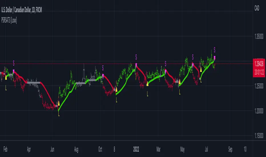
VHF-Adaptive T3 iTrend [Loxx]VHF-Adaptive T3 iTrend is an iTrend indicator with T3 smoothing and Vertical Horizontal Filter Adaptive period input. iTrend is used to determine where the trend starts and ends. You'll notice that the noise filter on this one is extreme. Adjust the period inputs accordingly to suit your take and your backtest requirements. This is also useful for scalping lower timeframes. Enjoy!
What is VHF Adaptive Period?
Vertical Horizontal Filter (VHF) was created by Adam White to identify trending and ranging markets. VHF measures the level of trend activity, similar to ADX DI. Vertical Horizontal Filter does not, itself, generate trading signals, but determines whether signals are taken from trend or momentum indicators. Using this trend information, one is then able to derive an average cycle length.
What is the T3 moving average?
Better Moving Averages Tim Tillson
November 1, 1998
Tim Tillson is a software project manager at Hewlett-Packard, with degrees in Mathematics and Computer Science. He has privately traded options and equities for 15 years.
Introduction
"Digital filtering includes the process of smoothing, predicting, differentiating, integrating, separation of signals, and removal of noise from a signal. Thus many people who do such things are actually using digital filters without realizing that they are; being unacquainted with the theory, they neither understand what they have done nor the possibilities of what they might have done."
This quote from R. W. Hamming applies to the vast majority of indicators in technical analysis . Moving averages, be they simple, weighted, or exponential, are lowpass filters; low frequency components in the signal pass through with little attenuation, while high frequencies are severely reduced.
"Oscillator" type indicators (such as MACD , Momentum, Relative Strength Index ) are another type of digital filter called a differentiator.
Tushar Chande has observed that many popular oscillators are highly correlated, which is sensible because they are trying to measure the rate of change of the underlying time series, i.e., are trying to be the first and second derivatives we all learned about in Calculus.
We use moving averages (lowpass filters) in technical analysis to remove the random noise from a time series, to discern the underlying trend or to determine prices at which we will take action. A perfect moving average would have two attributes:
It would be smooth, not sensitive to random noise in the underlying time series. Another way of saying this is that its derivative would not spuriously alternate between positive and negative values.
It would not lag behind the time series it is computed from. Lag, of course, produces late buy or sell signals that kill profits.
The only way one can compute a perfect moving average is to have knowledge of the future, and if we had that, we would buy one lottery ticket a week rather than trade!
Having said this, we can still improve on the conventional simple, weighted, or exponential moving averages. Here's how:
Two Interesting Moving Averages
We will examine two benchmark moving averages based on Linear Regression analysis.
In both cases, a Linear Regression line of length n is fitted to price data.
I call the first moving average ILRS, which stands for Integral of Linear Regression Slope. One simply integrates the slope of a linear regression line as it is successively fitted in a moving window of length n across the data, with the constant of integration being a simple moving average of the first n points. Put another way, the derivative of ILRS is the linear regression slope. Note that ILRS is not the same as a SMA ( simple moving average ) of length n, which is actually the midpoint of the linear regression line as it moves across the data.
We can measure the lag of moving averages with respect to a linear trend by computing how they behave when the input is a line with unit slope. Both SMA (n) and ILRS(n) have lag of n/2, but ILRS is much smoother than SMA .
Our second benchmark moving average is well known, called EPMA or End Point Moving Average. It is the endpoint of the linear regression line of length n as it is fitted across the data. EPMA hugs the data more closely than a simple or exponential moving average of the same length. The price we pay for this is that it is much noisier (less smooth) than ILRS, and it also has the annoying property that it overshoots the data when linear trends are present.
However, EPMA has a lag of 0 with respect to linear input! This makes sense because a linear regression line will fit linear input perfectly, and the endpoint of the LR line will be on the input line.
These two moving averages frame the tradeoffs that we are facing. On one extreme we have ILRS, which is very smooth and has considerable phase lag. EPMA has 0 phase lag, but is too noisy and overshoots. We would like to construct a better moving average which is as smooth as ILRS, but runs closer to where EPMA lies, without the overshoot.
A easy way to attempt this is to split the difference, i.e. use (ILRS(n)+EPMA(n))/2. This will give us a moving average (call it IE /2) which runs in between the two, has phase lag of n/4 but still inherits considerable noise from EPMA. IE /2 is inspirational, however. Can we build something that is comparable, but smoother? Figure 1 shows ILRS, EPMA, and IE /2.
Filter Techniques
Any thoughtful student of filter theory (or resolute experimenter) will have noticed that you can improve the smoothness of a filter by running it through itself multiple times, at the cost of increasing phase lag.
There is a complementary technique (called twicing by J.W. Tukey) which can be used to improve phase lag. If L stands for the operation of running data through a low pass filter, then twicing can be described by:
L' = L(time series) + L(time series - L(time series))
That is, we add a moving average of the difference between the input and the moving average to the moving average. This is algebraically equivalent to:
2L-L(L)
This is the Double Exponential Moving Average or DEMA , popularized by Patrick Mulloy in TASAC (January/February 1994).
In our taxonomy, DEMA has some phase lag (although it exponentially approaches 0) and is somewhat noisy, comparable to IE /2 indicator.
We will use these two techniques to construct our better moving average, after we explore the first one a little more closely.
Fixing Overshoot
An n-day EMA has smoothing constant alpha=2/(n+1) and a lag of (n-1)/2.
Thus EMA (3) has lag 1, and EMA (11) has lag 5. Figure 2 shows that, if I am willing to incur 5 days of lag, I get a smoother moving average if I run EMA (3) through itself 5 times than if I just take EMA (11) once.
This suggests that if EPMA and DEMA have 0 or low lag, why not run fast versions (eg DEMA (3)) through themselves many times to achieve a smooth result? The problem is that multiple runs though these filters increase their tendency to overshoot the data, giving an unusable result. This is because the amplitude response of DEMA and EPMA is greater than 1 at certain frequencies, giving a gain of much greater than 1 at these frequencies when run though themselves multiple times. Figure 3 shows DEMA (7) and EPMA(7) run through themselves 3 times. DEMA^3 has serious overshoot, and EPMA^3 is terrible.
The solution to the overshoot problem is to recall what we are doing with twicing:
DEMA (n) = EMA (n) + EMA (time series - EMA (n))
The second term is adding, in effect, a smooth version of the derivative to the EMA to achieve DEMA . The derivative term determines how hot the moving average's response to linear trends will be. We need to simply turn down the volume to achieve our basic building block:
EMA (n) + EMA (time series - EMA (n))*.7;
This is algebraically the same as:
EMA (n)*1.7-EMA( EMA (n))*.7;
I have chosen .7 as my volume factor, but the general formula (which I call "Generalized Dema") is:
GD (n,v) = EMA (n)*(1+v)-EMA( EMA (n))*v,
Where v ranges between 0 and 1. When v=0, GD is just an EMA , and when v=1, GD is DEMA . In between, GD is a cooler DEMA . By using a value for v less than 1 (I like .7), we cure the multiple DEMA overshoot problem, at the cost of accepting some additional phase delay. Now we can run GD through itself multiple times to define a new, smoother moving average T3 that does not overshoot the data:
T3(n) = GD ( GD ( GD (n)))
In filter theory parlance, T3 is a six-pole non-linear Kalman filter. Kalman filters are ones which use the error (in this case (time series - EMA (n)) to correct themselves. In Technical Analysis , these are called Adaptive Moving Averages; they track the time series more aggressively when it is making large moves.
Included
Bar coloring
Alerts
Signals
Loxx's Expanded Source Types
Buscar en scripts para "moving averages"
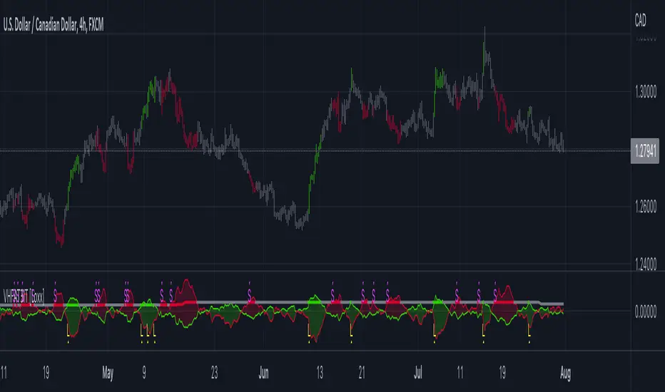
CFB-Adaptive CCI w/ T3 Smoothing [Loxx]CFB-Adaptive CCI w/ T3 Smoothing is a CCI indicator with adaptive period inputs and T3 smoothing. Jurik's Composite Fractal Behavior is used to created dynamic period input.
What is Composite Fractal Behavior ( CFB )?
All around you mechanisms adjust themselves to their environment. From simple thermostats that react to air temperature to computer chips in modern cars that respond to changes in engine temperature, r.p.m.'s, torque, and throttle position. It was only a matter of time before fast desktop computers applied the mathematics of self-adjustment to systems that trade the financial markets.
Unlike basic systems with fixed formulas, an adaptive system adjusts its own equations. For example, start with a basic channel breakout system that uses the highest closing price of the last N bars as a threshold for detecting breakouts on the up side. An adaptive and improved version of this system would adjust N according to market conditions, such as momentum, price volatility or acceleration.
Since many systems are based directly or indirectly on cycles, another useful measure of market condition is the periodic length of a price chart's dominant cycle, (DC), that cycle with the greatest influence on price action.
The utility of this new DC measure was noted by author Murray Ruggiero in the January '96 issue of Futures Magazine. In it. Mr. Ruggiero used it to adaptive adjust the value of N in a channel breakout system. He then simulated trading 15 years of D-Mark futures in order to compare its performance to a similar system that had a fixed optimal value of N. The adaptive version produced 20% more profit!
This DC index utilized the popular MESA algorithm (a formulation by John Ehlers adapted from Burg's maximum entropy algorithm, MEM). Unfortunately, the DC approach is problematic when the market has no real dominant cycle momentum, because the mathematics will produce a value whether or not one actually exists! Therefore, we developed a proprietary indicator that does not presuppose the presence of market cycles. It's called CFB (Composite Fractal Behavior) and it works well whether or not the market is cyclic.
CFB examines price action for a particular fractal pattern, categorizes them by size, and then outputs a composite fractal size index. This index is smooth, timely and accurate
Essentially, CFB reveals the length of the market's trending action time frame. Long trending activity produces a large CFB index and short choppy action produces a small index value. Investors have found many applications for CFB which involve scaling other existing technical indicators adaptively, on a bar-to-bar basis.
What is Jurik Volty used in the Juirk Filter?
One of the lesser known qualities of Juirk smoothing is that the Jurik smoothing process is adaptive. "Jurik Volty" (a sort of market volatility ) is what makes Jurik smoothing adaptive. The Jurik Volty calculation can be used as both a standalone indicator and to smooth other indicators that you wish to make adaptive.
What is the Jurik Moving Average?
Have you noticed how moving averages add some lag (delay) to your signals? ... especially when price gaps up or down in a big move, and you are waiting for your moving average to catch up? Wait no more! JMA eliminates this problem forever and gives you the best of both worlds: low lag and smooth lines.
Ideally, you would like a filtered signal to be both smooth and lag-free. Lag causes delays in your trades, and increasing lag in your indicators typically result in lower profits. In other words, late comers get what's left on the table after the feast has already begun.
What is the T3 moving average?
Better Moving Averages Tim Tillson
November 1, 1998
Tim Tillson is a software project manager at Hewlett-Packard, with degrees in Mathematics and Computer Science. He has privately traded options and equities for 15 years.
Introduction
"Digital filtering includes the process of smoothing, predicting, differentiating, integrating, separation of signals, and removal of noise from a signal. Thus many people who do such things are actually using digital filters without realizing that they are; being unacquainted with the theory, they neither understand what they have done nor the possibilities of what they might have done."
This quote from R. W. Hamming applies to the vast majority of indicators in technical analysis . Moving averages, be they simple, weighted, or exponential, are lowpass filters; low frequency components in the signal pass through with little attenuation, while high frequencies are severely reduced.
"Oscillator" type indicators (such as MACD , Momentum, Relative Strength Index ) are another type of digital filter called a differentiator.
Tushar Chande has observed that many popular oscillators are highly correlated, which is sensible because they are trying to measure the rate of change of the underlying time series, i.e., are trying to be the first and second derivatives we all learned about in Calculus.
We use moving averages (lowpass filters) in technical analysis to remove the random noise from a time series, to discern the underlying trend or to determine prices at which we will take action. A perfect moving average would have two attributes:
It would be smooth, not sensitive to random noise in the underlying time series. Another way of saying this is that its derivative would not spuriously alternate between positive and negative values.
It would not lag behind the time series it is computed from. Lag, of course, produces late buy or sell signals that kill profits.
The only way one can compute a perfect moving average is to have knowledge of the future, and if we had that, we would buy one lottery ticket a week rather than trade!
Having said this, we can still improve on the conventional simple, weighted, or exponential moving averages. Here's how:
Two Interesting Moving Averages
We will examine two benchmark moving averages based on Linear Regression analysis.
In both cases, a Linear Regression line of length n is fitted to price data.
I call the first moving average ILRS, which stands for Integral of Linear Regression Slope. One simply integrates the slope of a linear regression line as it is successively fitted in a moving window of length n across the data, with the constant of integration being a simple moving average of the first n points. Put another way, the derivative of ILRS is the linear regression slope. Note that ILRS is not the same as a SMA ( simple moving average ) of length n, which is actually the midpoint of the linear regression line as it moves across the data.
We can measure the lag of moving averages with respect to a linear trend by computing how they behave when the input is a line with unit slope. Both SMA (n) and ILRS(n) have lag of n/2, but ILRS is much smoother than SMA .
Our second benchmark moving average is well known, called EPMA or End Point Moving Average. It is the endpoint of the linear regression line of length n as it is fitted across the data. EPMA hugs the data more closely than a simple or exponential moving average of the same length. The price we pay for this is that it is much noisier (less smooth) than ILRS, and it also has the annoying property that it overshoots the data when linear trends are present.
However, EPMA has a lag of 0 with respect to linear input! This makes sense because a linear regression line will fit linear input perfectly, and the endpoint of the LR line will be on the input line.
These two moving averages frame the tradeoffs that we are facing. On one extreme we have ILRS, which is very smooth and has considerable phase lag. EPMA has 0 phase lag, but is too noisy and overshoots. We would like to construct a better moving average which is as smooth as ILRS, but runs closer to where EPMA lies, without the overshoot.
A easy way to attempt this is to split the difference, i.e. use (ILRS(n)+EPMA(n))/2. This will give us a moving average (call it IE /2) which runs in between the two, has phase lag of n/4 but still inherits considerable noise from EPMA. IE /2 is inspirational, however. Can we build something that is comparable, but smoother? Figure 1 shows ILRS, EPMA, and IE /2.
Filter Techniques
Any thoughtful student of filter theory (or resolute experimenter) will have noticed that you can improve the smoothness of a filter by running it through itself multiple times, at the cost of increasing phase lag.
There is a complementary technique (called twicing by J.W. Tukey) which can be used to improve phase lag. If L stands for the operation of running data through a low pass filter, then twicing can be described by:
L' = L(time series) + L(time series - L(time series))
That is, we add a moving average of the difference between the input and the moving average to the moving average. This is algebraically equivalent to:
2L-L(L)
This is the Double Exponential Moving Average or DEMA , popularized by Patrick Mulloy in TASAC (January/February 1994).
In our taxonomy, DEMA has some phase lag (although it exponentially approaches 0) and is somewhat noisy, comparable to IE /2 indicator.
We will use these two techniques to construct our better moving average, after we explore the first one a little more closely.
Fixing Overshoot
An n-day EMA has smoothing constant alpha=2/(n+1) and a lag of (n-1)/2.
Thus EMA (3) has lag 1, and EMA (11) has lag 5. Figure 2 shows that, if I am willing to incur 5 days of lag, I get a smoother moving average if I run EMA (3) through itself 5 times than if I just take EMA (11) once.
This suggests that if EPMA and DEMA have 0 or low lag, why not run fast versions (eg DEMA (3)) through themselves many times to achieve a smooth result? The problem is that multiple runs though these filters increase their tendency to overshoot the data, giving an unusable result. This is because the amplitude response of DEMA and EPMA is greater than 1 at certain frequencies, giving a gain of much greater than 1 at these frequencies when run though themselves multiple times. Figure 3 shows DEMA (7) and EPMA(7) run through themselves 3 times. DEMA^3 has serious overshoot, and EPMA^3 is terrible.
The solution to the overshoot problem is to recall what we are doing with twicing:
DEMA (n) = EMA (n) + EMA (time series - EMA (n))
The second term is adding, in effect, a smooth version of the derivative to the EMA to achieve DEMA . The derivative term determines how hot the moving average's response to linear trends will be. We need to simply turn down the volume to achieve our basic building block:
EMA (n) + EMA (time series - EMA (n))*.7;
This is algebraically the same as:
EMA (n)*1.7-EMA( EMA (n))*.7;
I have chosen .7 as my volume factor, but the general formula (which I call "Generalized Dema") is:
GD (n,v) = EMA (n)*(1+v)-EMA( EMA (n))*v,
Where v ranges between 0 and 1. When v=0, GD is just an EMA , and when v=1, GD is DEMA . In between, GD is a cooler DEMA . By using a value for v less than 1 (I like .7), we cure the multiple DEMA overshoot problem, at the cost of accepting some additional phase delay. Now we can run GD through itself multiple times to define a new, smoother moving average T3 that does not overshoot the data:
T3(n) = GD ( GD ( GD (n)))
In filter theory parlance, T3 is a six-pole non-linear Kalman filter. Kalman filters are ones which use the error (in this case (time series - EMA (n)) to correct themselves. In Technical Analysis , these are called Adaptive Moving Averages; they track the time series more aggressively when it is making large moves.
Included:
Bar coloring
Signals
Alerts

STD-Adaptive T3 Channel w/ Ehlers Swiss Army Knife Mod. [Loxx]STD-Adaptive T3 Channel w/ Ehlers Swiss Army Knife Mod. is an adaptive T3 indicator using standard deviation adaptivity and Ehlers Swiss Army Knife indicator to adjust the alpha value of the T3 calculation. This helps identify trends and reduce noise. In addition. I've included a Keltner Channel to show reversal/exhaustion zones.
What is the Swiss Army Knife Indicator?
John Ehlers explains the calculation here: www.mesasoftware.com
What is the T3 moving average?
Better Moving Averages Tim Tillson
November 1, 1998
Tim Tillson is a software project manager at Hewlett-Packard, with degrees in Mathematics and Computer Science. He has privately traded options and equities for 15 years.
Introduction
"Digital filtering includes the process of smoothing, predicting, differentiating, integrating, separation of signals, and removal of noise from a signal. Thus many people who do such things are actually using digital filters without realizing that they are; being unacquainted with the theory, they neither understand what they have done nor the possibilities of what they might have done."
This quote from R. W. Hamming applies to the vast majority of indicators in technical analysis . Moving averages, be they simple, weighted, or exponential, are lowpass filters; low frequency components in the signal pass through with little attenuation, while high frequencies are severely reduced.
"Oscillator" type indicators (such as MACD , Momentum, Relative Strength Index ) are another type of digital filter called a differentiator.
Tushar Chande has observed that many popular oscillators are highly correlated, which is sensible because they are trying to measure the rate of change of the underlying time series, i.e., are trying to be the first and second derivatives we all learned about in Calculus.
We use moving averages (lowpass filters) in technical analysis to remove the random noise from a time series, to discern the underlying trend or to determine prices at which we will take action. A perfect moving average would have two attributes:
It would be smooth, not sensitive to random noise in the underlying time series. Another way of saying this is that its derivative would not spuriously alternate between positive and negative values.
It would not lag behind the time series it is computed from. Lag, of course, produces late buy or sell signals that kill profits.
The only way one can compute a perfect moving average is to have knowledge of the future, and if we had that, we would buy one lottery ticket a week rather than trade!
Having said this, we can still improve on the conventional simple, weighted, or exponential moving averages. Here's how:
Two Interesting Moving Averages
We will examine two benchmark moving averages based on Linear Regression analysis.
In both cases, a Linear Regression line of length n is fitted to price data.
I call the first moving average ILRS, which stands for Integral of Linear Regression Slope. One simply integrates the slope of a linear regression line as it is successively fitted in a moving window of length n across the data, with the constant of integration being a simple moving average of the first n points. Put another way, the derivative of ILRS is the linear regression slope. Note that ILRS is not the same as a SMA ( simple moving average ) of length n, which is actually the midpoint of the linear regression line as it moves across the data.
We can measure the lag of moving averages with respect to a linear trend by computing how they behave when the input is a line with unit slope. Both SMA (n) and ILRS(n) have lag of n/2, but ILRS is much smoother than SMA .
Our second benchmark moving average is well known, called EPMA or End Point Moving Average. It is the endpoint of the linear regression line of length n as it is fitted across the data. EPMA hugs the data more closely than a simple or exponential moving average of the same length. The price we pay for this is that it is much noisier (less smooth) than ILRS, and it also has the annoying property that it overshoots the data when linear trends are present.
However, EPMA has a lag of 0 with respect to linear input! This makes sense because a linear regression line will fit linear input perfectly, and the endpoint of the LR line will be on the input line.
These two moving averages frame the tradeoffs that we are facing. On one extreme we have ILRS, which is very smooth and has considerable phase lag. EPMA has 0 phase lag, but is too noisy and overshoots. We would like to construct a better moving average which is as smooth as ILRS, but runs closer to where EPMA lies, without the overshoot.
A easy way to attempt this is to split the difference, i.e. use (ILRS(n)+EPMA(n))/2. This will give us a moving average (call it IE /2) which runs in between the two, has phase lag of n/4 but still inherits considerable noise from EPMA. IE /2 is inspirational, however. Can we build something that is comparable, but smoother? Figure 1 shows ILRS, EPMA, and IE /2.
Filter Techniques
Any thoughtful student of filter theory (or resolute experimenter) will have noticed that you can improve the smoothness of a filter by running it through itself multiple times, at the cost of increasing phase lag.
There is a complementary technique (called twicing by J.W. Tukey) which can be used to improve phase lag. If L stands for the operation of running data through a low pass filter, then twicing can be described by:
L' = L(time series) + L(time series - L(time series))
That is, we add a moving average of the difference between the input and the moving average to the moving average. This is algebraically equivalent to:
2L-L(L)
This is the Double Exponential Moving Average or DEMA , popularized by Patrick Mulloy in TASAC (January/February 1994).
In our taxonomy, DEMA has some phase lag (although it exponentially approaches 0) and is somewhat noisy, comparable to IE /2 indicator.
We will use these two techniques to construct our better moving average, after we explore the first one a little more closely.
Fixing Overshoot
An n-day EMA has smoothing constant alpha=2/(n+1) and a lag of (n-1)/2.
Thus EMA (3) has lag 1, and EMA (11) has lag 5. Figure 2 shows that, if I am willing to incur 5 days of lag, I get a smoother moving average if I run EMA (3) through itself 5 times than if I just take EMA (11) once.
This suggests that if EPMA and DEMA have 0 or low lag, why not run fast versions (eg DEMA (3)) through themselves many times to achieve a smooth result? The problem is that multiple runs though these filters increase their tendency to overshoot the data, giving an unusable result. This is because the amplitude response of DEMA and EPMA is greater than 1 at certain frequencies, giving a gain of much greater than 1 at these frequencies when run though themselves multiple times. Figure 3 shows DEMA (7) and EPMA(7) run through themselves 3 times. DEMA^3 has serious overshoot, and EPMA^3 is terrible.
The solution to the overshoot problem is to recall what we are doing with twicing:
DEMA (n) = EMA (n) + EMA (time series - EMA (n))
The second term is adding, in effect, a smooth version of the derivative to the EMA to achieve DEMA . The derivative term determines how hot the moving average's response to linear trends will be. We need to simply turn down the volume to achieve our basic building block:
EMA (n) + EMA (time series - EMA (n))*.7;
This is algebraically the same as:
EMA (n)*1.7-EMA( EMA (n))*.7;
I have chosen .7 as my volume factor, but the general formula (which I call "Generalized Dema") is:
GD (n,v) = EMA (n)*(1+v)-EMA( EMA (n))*v,
Where v ranges between 0 and 1. When v=0, GD is just an EMA , and when v=1, GD is DEMA . In between, GD is a cooler DEMA . By using a value for v less than 1 (I like .7), we cure the multiple DEMA overshoot problem, at the cost of accepting some additional phase delay. Now we can run GD through itself multiple times to define a new, smoother moving average T3 that does not overshoot the data:
T3(n) = GD ( GD ( GD (n)))
In filter theory parlance, T3 is a six-pole non-linear Kalman filter. Kalman filters are ones which use the error (in this case (time series - EMA (n)) to correct themselves. In Technical Analysis , these are called Adaptive Moving Averages; they track the time series more aggressively when it is making large moves.
Included:
Bar coloring
Signals
Alerts
Loxx's Expanded Source Types
T3 Velocity [Loxx]T3 Velocity is a simple velocity indicator using T3 moving average that uses gradient colors to better identify trends.
What is the T3 moving average?
Better Moving Averages Tim Tillson
November 1, 1998
Tim Tillson is a software project manager at Hewlett-Packard, with degrees in Mathematics and Computer Science. He has privately traded options and equities for 15 years.
Introduction
"Digital filtering includes the process of smoothing, predicting, differentiating, integrating, separation of signals, and removal of noise from a signal. Thus many people who do such things are actually using digital filters without realizing that they are; being unacquainted with the theory, they neither understand what they have done nor the possibilities of what they might have done."
This quote from R. W. Hamming applies to the vast majority of indicators in technical analysis . Moving averages, be they simple, weighted, or exponential, are lowpass filters; low frequency components in the signal pass through with little attenuation, while high frequencies are severely reduced.
"Oscillator" type indicators (such as MACD , Momentum, Relative Strength Index ) are another type of digital filter called a differentiator.
Tushar Chande has observed that many popular oscillators are highly correlated, which is sensible because they are trying to measure the rate of change of the underlying time series, i.e., are trying to be the first and second derivatives we all learned about in Calculus.
We use moving averages (lowpass filters) in technical analysis to remove the random noise from a time series, to discern the underlying trend or to determine prices at which we will take action. A perfect moving average would have two attributes:
It would be smooth, not sensitive to random noise in the underlying time series. Another way of saying this is that its derivative would not spuriously alternate between positive and negative values.
It would not lag behind the time series it is computed from. Lag, of course, produces late buy or sell signals that kill profits.
The only way one can compute a perfect moving average is to have knowledge of the future, and if we had that, we would buy one lottery ticket a week rather than trade!
Having said this, we can still improve on the conventional simple, weighted, or exponential moving averages. Here's how:
Two Interesting Moving Averages
We will examine two benchmark moving averages based on Linear Regression analysis.
In both cases, a Linear Regression line of length n is fitted to price data.
I call the first moving average ILRS, which stands for Integral of Linear Regression Slope. One simply integrates the slope of a linear regression line as it is successively fitted in a moving window of length n across the data, with the constant of integration being a simple moving average of the first n points. Put another way, the derivative of ILRS is the linear regression slope. Note that ILRS is not the same as a SMA ( simple moving average ) of length n, which is actually the midpoint of the linear regression line as it moves across the data.
We can measure the lag of moving averages with respect to a linear trend by computing how they behave when the input is a line with unit slope. Both SMA (n) and ILRS(n) have lag of n/2, but ILRS is much smoother than SMA .
Our second benchmark moving average is well known, called EPMA or End Point Moving Average. It is the endpoint of the linear regression line of length n as it is fitted across the data. EPMA hugs the data more closely than a simple or exponential moving average of the same length. The price we pay for this is that it is much noisier (less smooth) than ILRS, and it also has the annoying property that it overshoots the data when linear trends are present.
However, EPMA has a lag of 0 with respect to linear input! This makes sense because a linear regression line will fit linear input perfectly, and the endpoint of the LR line will be on the input line.
These two moving averages frame the tradeoffs that we are facing. On one extreme we have ILRS, which is very smooth and has considerable phase lag. EPMA has 0 phase lag, but is too noisy and overshoots. We would like to construct a better moving average which is as smooth as ILRS, but runs closer to where EPMA lies, without the overshoot.
A easy way to attempt this is to split the difference, i.e. use (ILRS(n)+EPMA(n))/2. This will give us a moving average (call it IE /2) which runs in between the two, has phase lag of n/4 but still inherits considerable noise from EPMA. IE /2 is inspirational, however. Can we build something that is comparable, but smoother? Figure 1 shows ILRS, EPMA, and IE /2.
Filter Techniques
Any thoughtful student of filter theory (or resolute experimenter) will have noticed that you can improve the smoothness of a filter by running it through itself multiple times, at the cost of increasing phase lag.
There is a complementary technique (called twicing by J.W. Tukey) which can be used to improve phase lag. If L stands for the operation of running data through a low pass filter, then twicing can be described by:
L' = L(time series) + L(time series - L(time series))
That is, we add a moving average of the difference between the input and the moving average to the moving average. This is algebraically equivalent to:
2L-L(L)
This is the Double Exponential Moving Average or DEMA , popularized by Patrick Mulloy in TASAC (January/February 1994).
In our taxonomy, DEMA has some phase lag (although it exponentially approaches 0) and is somewhat noisy, comparable to IE /2 indicator.
We will use these two techniques to construct our better moving average, after we explore the first one a little more closely.
Fixing Overshoot
An n-day EMA has smoothing constant alpha=2/(n+1) and a lag of (n-1)/2.
Thus EMA (3) has lag 1, and EMA (11) has lag 5. Figure 2 shows that, if I am willing to incur 5 days of lag, I get a smoother moving average if I run EMA (3) through itself 5 times than if I just take EMA (11) once.
This suggests that if EPMA and DEMA have 0 or low lag, why not run fast versions (eg DEMA (3)) through themselves many times to achieve a smooth result? The problem is that multiple runs though these filters increase their tendency to overshoot the data, giving an unusable result. This is because the amplitude response of DEMA and EPMA is greater than 1 at certain frequencies, giving a gain of much greater than 1 at these frequencies when run though themselves multiple times. Figure 3 shows DEMA (7) and EPMA(7) run through themselves 3 times. DEMA^3 has serious overshoot, and EPMA^3 is terrible.
The solution to the overshoot problem is to recall what we are doing with twicing:
DEMA (n) = EMA (n) + EMA (time series - EMA (n))
The second term is adding, in effect, a smooth version of the derivative to the EMA to achieve DEMA . The derivative term determines how hot the moving average's response to linear trends will be. We need to simply turn down the volume to achieve our basic building block:
EMA (n) + EMA (time series - EMA (n))*.7;
This is algebraically the same as:
EMA (n)*1.7-EMA( EMA (n))*.7;
I have chosen .7 as my volume factor, but the general formula (which I call "Generalized Dema") is:
GD (n,v) = EMA (n)*(1+v)-EMA( EMA (n))*v,
Where v ranges between 0 and 1. When v=0, GD is just an EMA , and when v=1, GD is DEMA . In between, GD is a cooler DEMA . By using a value for v less than 1 (I like .7), we cure the multiple DEMA overshoot problem, at the cost of accepting some additional phase delay. Now we can run GD through itself multiple times to define a new, smoother moving average T3 that does not overshoot the data:
T3(n) = GD ( GD ( GD (n)))
In filter theory parlance, T3 is a six-pole non-linear Kalman filter. Kalman filters are ones which use the error (in this case (time series - EMA (n)) to correct themselves. In Technical Analysis , these are called Adaptive Moving Averages; they track the time series more aggressively when it is making large moves.
Included:
Bar coloring
Signals
Alerts
Loxx's Expanded Source Types

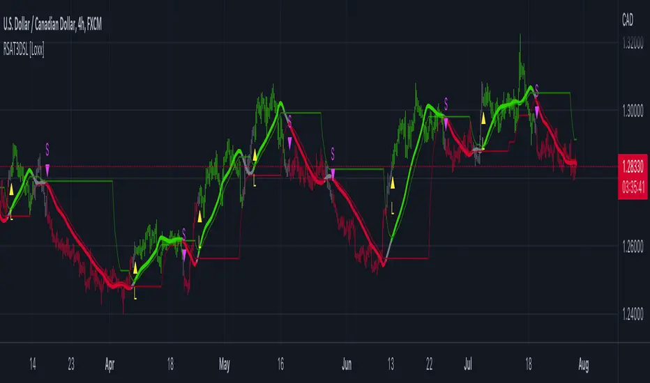
R-squared Adaptive T3 w/ DSL [Loxx]R-squared Adaptive T3 w/ DSL is the following T3 indicator but with Discontinued Signal Lines added to reduce noise and thereby increase signal accuracy. This adaptation makes this indicator lower TF scalp friendly.
What is R-squared Adaptive?
One tool available in forecasting the trendiness of the breakout is the coefficient of determination ( R-squared ), a statistical measurement.
The R-squared indicates linear strength between the security's price (the Y - axis) and time (the X - axis). The R-squared is the percentage of squared error that the linear regression can eliminate if it were used as the predictor instead of the mean value. If the R-squared were 0.99, then the linear regression would eliminate 99% of the error for prediction versus predicting closing prices using a simple moving average .
R-squared is used here to derive a T3 factor used to modify price before passing price through a six-pole non-linear Kalman filter.
What is the T3 moving average?
Better Moving Averages Tim Tillson
November 1, 1998
Tim Tillson is a software project manager at Hewlett-Packard, with degrees in Mathematics and Computer Science. He has privately traded options and equities for 15 years.
Introduction
"Digital filtering includes the process of smoothing, predicting, differentiating, integrating, separation of signals, and removal of noise from a signal. Thus many people who do such things are actually using digital filters without realizing that they are; being unacquainted with the theory, they neither understand what they have done nor the possibilities of what they might have done."
This quote from R. W. Hamming applies to the vast majority of indicators in technical analysis . Moving averages, be they simple, weighted, or exponential, are lowpass filters; low frequency components in the signal pass through with little attenuation, while high frequencies are severely reduced.
"Oscillator" type indicators (such as MACD , Momentum, Relative Strength Index ) are another type of digital filter called a differentiator.
Tushar Chande has observed that many popular oscillators are highly correlated, which is sensible because they are trying to measure the rate of change of the underlying time series, i.e., are trying to be the first and second derivatives we all learned about in Calculus.
We use moving averages (lowpass filters) in technical analysis to remove the random noise from a time series, to discern the underlying trend or to determine prices at which we will take action. A perfect moving average would have two attributes:
It would be smooth, not sensitive to random noise in the underlying time series. Another way of saying this is that its derivative would not spuriously alternate between positive and negative values.
It would not lag behind the time series it is computed from. Lag, of course, produces late buy or sell signals that kill profits.
The only way one can compute a perfect moving average is to have knowledge of the future, and if we had that, we would buy one lottery ticket a week rather than trade!
Having said this, we can still improve on the conventional simple, weighted, or exponential moving averages. Here's how:
Two Interesting Moving Averages
We will examine two benchmark moving averages based on Linear Regression analysis.
In both cases, a Linear Regression line of length n is fitted to price data.
I call the first moving average ILRS, which stands for Integral of Linear Regression Slope. One simply integrates the slope of a linear regression line as it is successively fitted in a moving window of length n across the data, with the constant of integration being a simple moving average of the first n points. Put another way, the derivative of ILRS is the linear regression slope. Note that ILRS is not the same as a SMA ( simple moving average ) of length n, which is actually the midpoint of the linear regression line as it moves across the data.
We can measure the lag of moving averages with respect to a linear trend by computing how they behave when the input is a line with unit slope. Both SMA (n) and ILRS(n) have lag of n/2, but ILRS is much smoother than SMA .
Our second benchmark moving average is well known, called EPMA or End Point Moving Average. It is the endpoint of the linear regression line of length n as it is fitted across the data. EPMA hugs the data more closely than a simple or exponential moving average of the same length. The price we pay for this is that it is much noisier (less smooth) than ILRS, and it also has the annoying property that it overshoots the data when linear trends are present.
However, EPMA has a lag of 0 with respect to linear input! This makes sense because a linear regression line will fit linear input perfectly, and the endpoint of the LR line will be on the input line.
These two moving averages frame the tradeoffs that we are facing. On one extreme we have ILRS, which is very smooth and has considerable phase lag. EPMA has 0 phase lag, but is too noisy and overshoots. We would like to construct a better moving average which is as smooth as ILRS, but runs closer to where EPMA lies, without the overshoot.
A easy way to attempt this is to split the difference, i.e. use (ILRS(n)+EPMA(n))/2. This will give us a moving average (call it IE /2) which runs in between the two, has phase lag of n/4 but still inherits considerable noise from EPMA. IE /2 is inspirational, however. Can we build something that is comparable, but smoother? Figure 1 shows ILRS, EPMA, and IE /2.
Filter Techniques
Any thoughtful student of filter theory (or resolute experimenter) will have noticed that you can improve the smoothness of a filter by running it through itself multiple times, at the cost of increasing phase lag.
There is a complementary technique (called twicing by J.W. Tukey) which can be used to improve phase lag. If L stands for the operation of running data through a low pass filter, then twicing can be described by:
L' = L(time series) + L(time series - L(time series))
That is, we add a moving average of the difference between the input and the moving average to the moving average. This is algebraically equivalent to:
2L-L(L)
This is the Double Exponential Moving Average or DEMA , popularized by Patrick Mulloy in TASAC (January/February 1994).
In our taxonomy, DEMA has some phase lag (although it exponentially approaches 0) and is somewhat noisy, comparable to IE /2 indicator.
We will use these two techniques to construct our better moving average, after we explore the first one a little more closely.
Fixing Overshoot
An n-day EMA has smoothing constant alpha=2/(n+1) and a lag of (n-1)/2.
Thus EMA (3) has lag 1, and EMA (11) has lag 5. Figure 2 shows that, if I am willing to incur 5 days of lag, I get a smoother moving average if I run EMA (3) through itself 5 times than if I just take EMA (11) once.
This suggests that if EPMA and DEMA have 0 or low lag, why not run fast versions (eg DEMA (3)) through themselves many times to achieve a smooth result? The problem is that multiple runs though these filters increase their tendency to overshoot the data, giving an unusable result. This is because the amplitude response of DEMA and EPMA is greater than 1 at certain frequencies, giving a gain of much greater than 1 at these frequencies when run though themselves multiple times. Figure 3 shows DEMA (7) and EPMA(7) run through themselves 3 times. DEMA^3 has serious overshoot, and EPMA^3 is terrible.
The solution to the overshoot problem is to recall what we are doing with twicing:
DEMA (n) = EMA (n) + EMA (time series - EMA (n))
The second term is adding, in effect, a smooth version of the derivative to the EMA to achieve DEMA . The derivative term determines how hot the moving average's response to linear trends will be. We need to simply turn down the volume to achieve our basic building block:
EMA (n) + EMA (time series - EMA (n))*.7;
This is algebraically the same as:
EMA (n)*1.7-EMA( EMA (n))*.7;
I have chosen .7 as my volume factor, but the general formula (which I call "Generalized Dema") is:
GD (n,v) = EMA (n)*(1+v)-EMA( EMA (n))*v,
Where v ranges between 0 and 1. When v=0, GD is just an EMA , and when v=1, GD is DEMA . In between, GD is a cooler DEMA . By using a value for v less than 1 (I like .7), we cure the multiple DEMA overshoot problem, at the cost of accepting some additional phase delay. Now we can run GD through itself multiple times to define a new, smoother moving average T3 that does not overshoot the data:
T3(n) = GD ( GD ( GD (n)))
In filter theory parlance, T3 is a six-pole non-linear Kalman filter. Kalman filters are ones which use the error (in this case (time series - EMA (n)) to correct themselves. In Technical Analysis , these are called Adaptive Moving Averages; they track the time series more aggressively when it is making large moves.
Included:
Bar coloring
Signals
Alerts
EMA and FEMA Signla/DSL smoothing
Loxx's Expanded Source Types
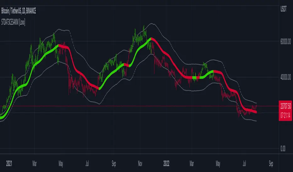
STD-Filterd, R-squared Adaptive T3 w/ Dynamic Zones [Loxx]STD-Filterd, R-squared Adaptive T3 w/ Dynamic Zones is a standard deviation filtered R-squared Adaptive T3 moving average with dynamic zones.
What is the T3 moving average?
Better Moving Averages Tim Tillson
November 1, 1998
Tim Tillson is a software project manager at Hewlett-Packard, with degrees in Mathematics and Computer Science. He has privately traded options and equities for 15 years.
Introduction
"Digital filtering includes the process of smoothing, predicting, differentiating, integrating, separation of signals, and removal of noise from a signal. Thus many people who do such things are actually using digital filters without realizing that they are; being unacquainted with the theory, they neither understand what they have done nor the possibilities of what they might have done."
This quote from R. W. Hamming applies to the vast majority of indicators in technical analysis . Moving averages, be they simple, weighted, or exponential, are lowpass filters; low frequency components in the signal pass through with little attenuation, while high frequencies are severely reduced.
"Oscillator" type indicators (such as MACD , Momentum, Relative Strength Index ) are another type of digital filter called a differentiator.
Tushar Chande has observed that many popular oscillators are highly correlated, which is sensible because they are trying to measure the rate of change of the underlying time series, i.e., are trying to be the first and second derivatives we all learned about in Calculus.
We use moving averages (lowpass filters) in technical analysis to remove the random noise from a time series, to discern the underlying trend or to determine prices at which we will take action. A perfect moving average would have two attributes:
It would be smooth, not sensitive to random noise in the underlying time series. Another way of saying this is that its derivative would not spuriously alternate between positive and negative values.
It would not lag behind the time series it is computed from. Lag, of course, produces late buy or sell signals that kill profits.
The only way one can compute a perfect moving average is to have knowledge of the future, and if we had that, we would buy one lottery ticket a week rather than trade!
Having said this, we can still improve on the conventional simple, weighted, or exponential moving averages. Here's how:
Two Interesting Moving Averages
We will examine two benchmark moving averages based on Linear Regression analysis.
In both cases, a Linear Regression line of length n is fitted to price data.
I call the first moving average ILRS, which stands for Integral of Linear Regression Slope. One simply integrates the slope of a linear regression line as it is successively fitted in a moving window of length n across the data, with the constant of integration being a simple moving average of the first n points. Put another way, the derivative of ILRS is the linear regression slope. Note that ILRS is not the same as a SMA ( simple moving average ) of length n, which is actually the midpoint of the linear regression line as it moves across the data.
We can measure the lag of moving averages with respect to a linear trend by computing how they behave when the input is a line with unit slope. Both SMA (n) and ILRS(n) have lag of n/2, but ILRS is much smoother than SMA .
Our second benchmark moving average is well known, called EPMA or End Point Moving Average. It is the endpoint of the linear regression line of length n as it is fitted across the data. EPMA hugs the data more closely than a simple or exponential moving average of the same length. The price we pay for this is that it is much noisier (less smooth) than ILRS, and it also has the annoying property that it overshoots the data when linear trends are present.
However, EPMA has a lag of 0 with respect to linear input! This makes sense because a linear regression line will fit linear input perfectly, and the endpoint of the LR line will be on the input line.
These two moving averages frame the tradeoffs that we are facing. On one extreme we have ILRS, which is very smooth and has considerable phase lag. EPMA has 0 phase lag, but is too noisy and overshoots. We would like to construct a better moving average which is as smooth as ILRS, but runs closer to where EPMA lies, without the overshoot.
A easy way to attempt this is to split the difference, i.e. use (ILRS(n)+EPMA(n))/2. This will give us a moving average (call it IE /2) which runs in between the two, has phase lag of n/4 but still inherits considerable noise from EPMA. IE /2 is inspirational, however. Can we build something that is comparable, but smoother? Figure 1 shows ILRS, EPMA, and IE /2.
Filter Techniques
Any thoughtful student of filter theory (or resolute experimenter) will have noticed that you can improve the smoothness of a filter by running it through itself multiple times, at the cost of increasing phase lag.
There is a complementary technique (called twicing by J.W. Tukey) which can be used to improve phase lag. If L stands for the operation of running data through a low pass filter, then twicing can be described by:
L' = L(time series) + L(time series - L(time series))
That is, we add a moving average of the difference between the input and the moving average to the moving average. This is algebraically equivalent to:
2L-L(L)
This is the Double Exponential Moving Average or DEMA , popularized by Patrick Mulloy in TASAC (January/February 1994).
In our taxonomy, DEMA has some phase lag (although it exponentially approaches 0) and is somewhat noisy, comparable to IE /2 indicator.
We will use these two techniques to construct our better moving average, after we explore the first one a little more closely.
Fixing Overshoot
An n-day EMA has smoothing constant alpha=2/(n+1) and a lag of (n-1)/2.
Thus EMA (3) has lag 1, and EMA (11) has lag 5. Figure 2 shows that, if I am willing to incur 5 days of lag, I get a smoother moving average if I run EMA (3) through itself 5 times than if I just take EMA (11) once.
This suggests that if EPMA and DEMA have 0 or low lag, why not run fast versions (eg DEMA (3)) through themselves many times to achieve a smooth result? The problem is that multiple runs though these filters increase their tendency to overshoot the data, giving an unusable result. This is because the amplitude response of DEMA and EPMA is greater than 1 at certain frequencies, giving a gain of much greater than 1 at these frequencies when run though themselves multiple times. Figure 3 shows DEMA (7) and EPMA(7) run through themselves 3 times. DEMA^3 has serious overshoot, and EPMA^3 is terrible.
The solution to the overshoot problem is to recall what we are doing with twicing:
DEMA (n) = EMA (n) + EMA (time series - EMA (n))
The second term is adding, in effect, a smooth version of the derivative to the EMA to achieve DEMA . The derivative term determines how hot the moving average's response to linear trends will be. We need to simply turn down the volume to achieve our basic building block:
EMA (n) + EMA (time series - EMA (n))*.7;
This is algebraically the same as:
EMA (n)*1.7-EMA( EMA (n))*.7;
I have chosen .7 as my volume factor, but the general formula (which I call "Generalized Dema") is:
GD (n,v) = EMA (n)*(1+v)-EMA( EMA (n))*v,
Where v ranges between 0 and 1. When v=0, GD is just an EMA , and when v=1, GD is DEMA . In between, GD is a cooler DEMA . By using a value for v less than 1 (I like .7), we cure the multiple DEMA overshoot problem, at the cost of accepting some additional phase delay. Now we can run GD through itself multiple times to define a new, smoother moving average T3 that does not overshoot the data:
T3(n) = GD ( GD ( GD (n)))
In filter theory parlance, T3 is a six-pole non-linear Kalman filter. Kalman filters are ones which use the error (in this case (time series - EMA (n)) to correct themselves. In Technical Analysis , these are called Adaptive Moving Averages; they track the time series more aggressively when it is making large moves.
What is R-squared Adaptive?
One tool available in forecasting the trendiness of the breakout is the coefficient of determination ( R-squared ), a statistical measurement.
The R-squared indicates linear strength between the security's price (the Y - axis) and time (the X - axis). The R-squared is the percentage of squared error that the linear regression can eliminate if it were used as the predictor instead of the mean value. If the R-squared were 0.99, then the linear regression would eliminate 99% of the error for prediction versus predicting closing prices using a simple moving average .
R-squared is used here to derive a T3 factor used to modify price before passing price through a six-pole non-linear Kalman filter.
What are Dynamic Zones?
As explained in "Stocks & Commodities V15:7 (306-310): Dynamic Zones by Leo Zamansky, Ph .D., and David Stendahl"
Most indicators use a fixed zone for buy and sell signals. Here’ s a concept based on zones that are responsive to past levels of the indicator.
One approach to active investing employs the use of oscillators to exploit tradable market trends. This investing style follows a very simple form of logic: Enter the market only when an oscillator has moved far above or below traditional trading lev- els. However, these oscillator- driven systems lack the ability to evolve with the market because they use fixed buy and sell zones. Traders typically use one set of buy and sell zones for a bull market and substantially different zones for a bear market. And therein lies the problem.
Once traders begin introducing their market opinions into trading equations, by changing the zones, they negate the system’s mechanical nature. The objective is to have a system automatically define its own buy and sell zones and thereby profitably trade in any market — bull or bear. Dynamic zones offer a solution to the problem of fixed buy and sell zones for any oscillator-driven system.
An indicator’s extreme levels can be quantified using statistical methods. These extreme levels are calculated for a certain period and serve as the buy and sell zones for a trading system. The repetition of this statistical process for every value of the indicator creates values that become the dynamic zones. The zones are calculated in such a way that the probability of the indicator value rising above, or falling below, the dynamic zones is equal to a given probability input set by the trader.
To better understand dynamic zones, let's first describe them mathematically and then explain their use. The dynamic zones definition:
Find V such that:
For dynamic zone buy: P{X <= V}=P1
For dynamic zone sell: P{X >= V}=P2
where P1 and P2 are the probabilities set by the trader, X is the value of the indicator for the selected period and V represents the value of the dynamic zone.
The probability input P1 and P2 can be adjusted by the trader to encompass as much or as little data as the trader would like. The smaller the probability, the fewer data values above and below the dynamic zones. This translates into a wider range between the buy and sell zones. If a 10% probability is used for P1 and P2, only those data values that make up the top 10% and bottom 10% for an indicator are used in the construction of the zones. Of the values, 80% will fall between the two extreme levels. Because dynamic zone levels are penetrated so infrequently, when this happens, traders know that the market has truly moved into overbought or oversold territory.
Calculating the Dynamic Zones
The algorithm for the dynamic zones is a series of steps. First, decide the value of the lookback period t. Next, decide the value of the probability Pbuy for buy zone and value of the probability Psell for the sell zone.
For i=1, to the last lookback period, build the distribution f(x) of the price during the lookback period i. Then find the value Vi1 such that the probability of the price less than or equal to Vi1 during the lookback period i is equal to Pbuy. Find the value Vi2 such that the probability of the price greater or equal to Vi2 during the lookback period i is equal to Psell. The sequence of Vi1 for all periods gives the buy zone. The sequence of Vi2 for all periods gives the sell zone.
In the algorithm description, we have: Build the distribution f(x) of the price during the lookback period i. The distribution here is empirical namely, how many times a given value of x appeared during the lookback period. The problem is to find such x that the probability of a price being greater or equal to x will be equal to a probability selected by the user. Probability is the area under the distribution curve. The task is to find such value of x that the area under the distribution curve to the right of x will be equal to the probability selected by the user. That x is the dynamic zone.
Included:
Bar coloring
Signals
Alerts
Loxx's Expanded Source Types

Pips-Stepped, R-squared Adaptive T3 [Loxx]Pips-Stepped, R-squared Adaptive T3 is a a T3 moving average with optional adaptivity, trend following, and pip-stepping. This indicator also uses optional flat coloring to determine chops zones. This indicator is R-squared adaptive. This is also an experimental indicator.
What is the T3 moving average?
Better Moving Averages Tim Tillson
November 1, 1998
Tim Tillson is a software project manager at Hewlett-Packard, with degrees in Mathematics and Computer Science. He has privately traded options and equities for 15 years.
Introduction
"Digital filtering includes the process of smoothing, predicting, differentiating, integrating, separation of signals, and removal of noise from a signal. Thus many people who do such things are actually using digital filters without realizing that they are; being unacquainted with the theory, they neither understand what they have done nor the possibilities of what they might have done."
This quote from R. W. Hamming applies to the vast majority of indicators in technical analysis . Moving averages, be they simple, weighted, or exponential, are lowpass filters; low frequency components in the signal pass through with little attenuation, while high frequencies are severely reduced.
"Oscillator" type indicators (such as MACD , Momentum, Relative Strength Index ) are another type of digital filter called a differentiator.
Tushar Chande has observed that many popular oscillators are highly correlated, which is sensible because they are trying to measure the rate of change of the underlying time series, i.e., are trying to be the first and second derivatives we all learned about in Calculus.
We use moving averages (lowpass filters) in technical analysis to remove the random noise from a time series, to discern the underlying trend or to determine prices at which we will take action. A perfect moving average would have two attributes:
It would be smooth, not sensitive to random noise in the underlying time series. Another way of saying this is that its derivative would not spuriously alternate between positive and negative values.
It would not lag behind the time series it is computed from. Lag, of course, produces late buy or sell signals that kill profits.
The only way one can compute a perfect moving average is to have knowledge of the future, and if we had that, we would buy one lottery ticket a week rather than trade!
Having said this, we can still improve on the conventional simple, weighted, or exponential moving averages. Here's how:
Two Interesting Moving Averages
We will examine two benchmark moving averages based on Linear Regression analysis.
In both cases, a Linear Regression line of length n is fitted to price data.
I call the first moving average ILRS, which stands for Integral of Linear Regression Slope. One simply integrates the slope of a linear regression line as it is successively fitted in a moving window of length n across the data, with the constant of integration being a simple moving average of the first n points. Put another way, the derivative of ILRS is the linear regression slope. Note that ILRS is not the same as a SMA ( simple moving average ) of length n, which is actually the midpoint of the linear regression line as it moves across the data.
We can measure the lag of moving averages with respect to a linear trend by computing how they behave when the input is a line with unit slope. Both SMA (n) and ILRS(n) have lag of n/2, but ILRS is much smoother than SMA .
Our second benchmark moving average is well known, called EPMA or End Point Moving Average. It is the endpoint of the linear regression line of length n as it is fitted across the data. EPMA hugs the data more closely than a simple or exponential moving average of the same length. The price we pay for this is that it is much noisier (less smooth) than ILRS, and it also has the annoying property that it overshoots the data when linear trends are present.
However, EPMA has a lag of 0 with respect to linear input! This makes sense because a linear regression line will fit linear input perfectly, and the endpoint of the LR line will be on the input line.
These two moving averages frame the tradeoffs that we are facing. On one extreme we have ILRS, which is very smooth and has considerable phase lag. EPMA has 0 phase lag, but is too noisy and overshoots. We would like to construct a better moving average which is as smooth as ILRS, but runs closer to where EPMA lies, without the overshoot.
A easy way to attempt this is to split the difference, i.e. use (ILRS(n)+EPMA(n))/2. This will give us a moving average (call it IE /2) which runs in between the two, has phase lag of n/4 but still inherits considerable noise from EPMA. IE /2 is inspirational, however. Can we build something that is comparable, but smoother? Figure 1 shows ILRS, EPMA, and IE /2.
Filter Techniques
Any thoughtful student of filter theory (or resolute experimenter) will have noticed that you can improve the smoothness of a filter by running it through itself multiple times, at the cost of increasing phase lag.
There is a complementary technique (called twicing by J.W. Tukey) which can be used to improve phase lag. If L stands for the operation of running data through a low pass filter, then twicing can be described by:
L' = L(time series) + L(time series - L(time series))
That is, we add a moving average of the difference between the input and the moving average to the moving average. This is algebraically equivalent to:
2L-L(L)
This is the Double Exponential Moving Average or DEMA , popularized by Patrick Mulloy in TASAC (January/February 1994).
In our taxonomy, DEMA has some phase lag (although it exponentially approaches 0) and is somewhat noisy, comparable to IE /2 indicator.
We will use these two techniques to construct our better moving average, after we explore the first one a little more closely.
Fixing Overshoot
An n-day EMA has smoothing constant alpha=2/(n+1) and a lag of (n-1)/2.
Thus EMA (3) has lag 1, and EMA (11) has lag 5. Figure 2 shows that, if I am willing to incur 5 days of lag, I get a smoother moving average if I run EMA (3) through itself 5 times than if I just take EMA (11) once.
This suggests that if EPMA and DEMA have 0 or low lag, why not run fast versions (eg DEMA (3)) through themselves many times to achieve a smooth result? The problem is that multiple runs though these filters increase their tendency to overshoot the data, giving an unusable result. This is because the amplitude response of DEMA and EPMA is greater than 1 at certain frequencies, giving a gain of much greater than 1 at these frequencies when run though themselves multiple times. Figure 3 shows DEMA (7) and EPMA(7) run through themselves 3 times. DEMA^3 has serious overshoot, and EPMA^3 is terrible.
The solution to the overshoot problem is to recall what we are doing with twicing:
DEMA (n) = EMA (n) + EMA (time series - EMA (n))
The second term is adding, in effect, a smooth version of the derivative to the EMA to achieve DEMA . The derivative term determines how hot the moving average's response to linear trends will be. We need to simply turn down the volume to achieve our basic building block:
EMA (n) + EMA (time series - EMA (n))*.7;
This is algebraically the same as:
EMA (n)*1.7-EMA( EMA (n))*.7;
I have chosen .7 as my volume factor, but the general formula (which I call "Generalized Dema") is:
GD (n,v) = EMA (n)*(1+v)-EMA( EMA (n))*v,
Where v ranges between 0 and 1. When v=0, GD is just an EMA , and when v=1, GD is DEMA . In between, GD is a cooler DEMA . By using a value for v less than 1 (I like .7), we cure the multiple DEMA overshoot problem, at the cost of accepting some additional phase delay. Now we can run GD through itself multiple times to define a new, smoother moving average T3 that does not overshoot the data:
T3(n) = GD ( GD ( GD (n)))
In filter theory parlance, T3 is a six-pole non-linear Kalman filter. Kalman filters are ones which use the error (in this case (time series - EMA (n)) to correct themselves. In Technical Analysis , these are called Adaptive Moving Averages; they track the time series more aggressively when it is making large moves.
What is R-squared Adaptive?
One tool available in forecasting the trendiness of the breakout is the coefficient of determination (R-squared), a statistical measurement.
The R-squared indicates linear strength between the security's price (the Y - axis) and time (the X - axis). The R-squared is the percentage of squared error that the linear regression can eliminate if it were used as the predictor instead of the mean value. If the R-squared were 0.99, then the linear regression would eliminate 99% of the error for prediction versus predicting closing prices using a simple moving average.
R-squared is used here to derive a T3 factor used to modify price before passing price through a six-pole non-linear Kalman filter.
Included:
Bar coloring
Signals
Alerts
Flat coloring
FULL MA Optimization ScriptHello!
This script measures the performance of 10 moving averages and compares them!
Crossover and crossunders are both tested.
The tested moving averages include: TEMA, DEMA, EMA, SMA, ALMA, HMA, T3 Average, WMA, VWMA, LSMA.
You can select the length of the moving averages and the data source (I.E, close, open, ohlc4, etc.) and the script will calculate your selections!
For instance, if you select a length of 32 and a source of ohlc4 for crossovers, the script will assign the ten moving averages that length and data source and compare the performance for ohlc4 crossovers of the 32TEMA, 32DEMA, 32SMA, 32WMA, etc. If you select crossunder, the script will calculate the performance of ohlc4 crossunders of the same moving average lengths.
Moving average performances are listed in descending order (best to worst) and are categorized by tier: Upper-Tier, Mid-Tier, Lower-Tier. The Upper-Tier displays the three best performing averages relative to the MA length and data source, for the asset on the relevant chart timeframe. The Lower-Tier displays the three worst performing averages. The Mid-Tier displays the moving averages whose performance did not achieve a top three spot or a bottom three spot.
Also calculated is the moving average which achieved the highest cumulative gain/loss and the lowest cumulative gain/loss. Any asset and timeframe can be tested; the script recalculates relative to the chart timeframe. I added a "Benchmark Moving Average" free parameter and a "Custom Moving Average" free parameter. The two operate identically; you can set the length and data source of both for quick and simple comparison between differing average lengths and sources.
If "Crossover" is selected, the "(X Candles)" displayed on the tables reflects the average number of sessions the data source remains above a moving average following a crossover. If "Crossunder" is selected, the "(X Candles)" reflects the average number of sessions the data source remains below the moving average following a crossunder.
If "Crossover" is selected, the listed "X%" reflects the average percentage gain/loss following a source crossover of a moving average up until the source crosses back under the moving average. If "Crossunder" is selected, the listed "X%" reflects the average percentage gain/loss following a source crossunder of a moving average up until the source crosses back over the moving average.
If "Crossover" is selected, the listed "X Crosses" reflects the number of instances in which the source crossed over a moving average. If "Crossunder" is selected, the listed "X Crosses" reflects the number of instances in which the source crossed under a moving average.
Additional tooltips and instructions are included should you access the user input menu.
The moving averages can be plotted as a gradient (highest priced MA to lowest priced MA) alongside the best performing moving average. The moving averages can be plotted in full color, light color alongside the best performing average, or not plotted.
This script improves upon a similar script I have released:
I decided not to update the previous script. The previous script calculates crossovers only and, due to being less code intensive, calculates much quicker. If a user is concerned only with price crossovers, not crossunders, the original script is a better option! It's faster, making it the preferable choice!
This script "FULL MA Optimization" calculates crossovers/crossunders and incorporates additional plot styles. I ran into trouble a few times where the script was too large to run on TV. This script is not "slow", I suppose; however, calculations and parameter modifications take a bit longer than the original script!

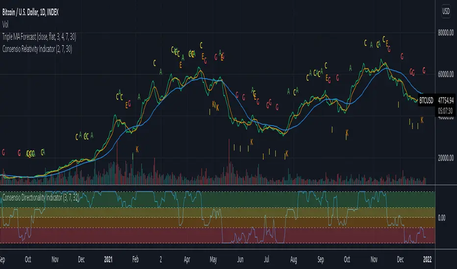
Consensio V2 - Relativity IndicatorThis indicator is based on Consensio Trading System by Tyler Jenks.
It is showing you in real-time when Relativity is changing. It will help you understand when you should probably lower your position, and when to strengthen your position, when to enter a market, and when to exit a market.
What is Relativity?
According to this trading system, you start by laying 3 Simple Moving Averages:
A Long-Term Moving Average (LTMA).
A Short-Term Moving Average (STMA).
A Price Moving Average (Price).
*The "Price" should be A relatively short Moving Average in order to reflect the current price.
When laying out those 3 Moving averages on top of each other, you discover 13 unique types of relationships:
Relativity A: Price > STMA, Price > LTMA, STMA > LTMA
Relativity B: Price = STMA, Price > LTMA, STMA > LTMA
Relativity C: Price < STMA, Price > LTMA, STMA > LTMA
Relativity D: Price < STMA, Price = LTMA, STMA > LTMA
Relativity E: Price < STMA, Price < LTMA, STMA > LTMA
Relativity F: Price < STMA, Price < LTMA, STMA = LTMA
Relativity G: Price < STMA, Price < LTMA, STMA < LTMA
Relativity H: Price = STMA, Price < LTMA, STMA < LTMA
Relativity I: Price > STMA, Price < LTMA, STMA < LTMA
Relativity J: Price > STMA, Price = LTMA, STMA < LTMA
Relativity K: Price > STMA, Price > LTMA, STMA < LTMA
Relativity L: Price > STMA, Price > LTMA, STMA = LTMA
Relativity M: Price = STMA, Price = LTMA, STMA = LTMA
So what's the big deal, you may ask?
For the market to go from Bullish State (type A) to Bearish state (type G), the Market must pass through Relativity B, C, D, E, F.
For the market to go from Bearish State (type G) to Bullish state (type A), the Market must pass through Relativity H, I, J, K, L.
Knowing This principle helps you better plan when to enter a market, and when to exit a market, when to Lower your position and when to strengthen your position.
Recommendations
Different Moving Averages may suit you better when trading different assets on different time periods. You can go into the indicator settings and change the Moving Averages values if needed.
When Moving Averages are consolidating, the Relativity can change direction more often. When this happens, it is better to wait for a stronger signal than to trade on every signal.
you should also use the "Consensio Directionality Indicator" to predict the directionality of the market. While using both of my Consensio indicators together, please make sure that the Moving Averages on both of them are set to the same values
Consensio Trading System encourages you to make decisions based on Moving Averages only. I highly recommend disabling "candle view" by switching to "line view" and changing the opacity of the line to 0.
JC MAs: SMA, WMA, EMA, DEMA, TEMA, ALMA, Hull, Kaufman, FractalThe best collection of moving averages anywhere. I know, because I searched, couldn't find the right collection, and so wrote it myself!
-------------------------------------------------------------------------------
Notable features that either aren't found anywhere else...or at least in one place:
-------------------------------------------------------------------------------
• The "Triple Exponential Moving Average", is actually that mathematically - rather than "three seperate EMA graphs", as is commonly found on Trading View.
• Includes exotic moving averages: Hull Moving Average (HMA), Kaufman's Adaptive Moving Average (KAMA), and Fractal Apaptive Moving Average (FrAMA).
• Each moving average has its own user-definable averaging length in DAYS, rather than an abstract "length". This is respected even for different graphing resolutions, and different chart views - even for the more exotic MAs.
• Days can be fractional.
• A master time resolution ("Timeframe") is also user-definable. And unlike most other moving average charts, this won't affect the internal "length" variable (specified days are still respected), it only changes the graphing resolution. You can also specify to use chart's resolution - which, as you know, is not very useful for moving averages - yet so many moving average scripts on Trading View don't let you specify otherwise.
• If every CPU cycle counts, you can set "days" to 0 to prevent a particular unneeded moving average from being calculated at all.
• Includes a custom moving average that is unique, if you're looking for a tiny edge in TA to beat everyone else looking at the same stuff: a customizable weighted blend of SMA, TEMA, HMA, KAMA, and FrMA. (Note: The weights for these blends don't have to add up to 100, they will self-level no matter what they add up to.)
• By default, the averages are color-coded according to rainbow order of light spectrum frequency, relative to approximate responsiveness to current price: Red (SMA) is the laziest, violet (FrAMA) is the most hyper, and green is in the middle.
-------------------------------------------------------------------------------
Contains the following moving averages, in order of responsiveness:
-------------------------------------------------------------------------------
• Simple Moving Average (SMA)
• Arnaud Legoux Moving Average (ALMA)
• Exponential Moving Average (EMA)
• Weighted Moving Average (WMA)
• Blend average of SMA and TEMA (JCBMA)
• Double Exponential Moving Average (DEMA)
• Triple Exponential Moving Average (TEMA)
• Hull Moving Average (HMA)
• Kaufman's Adaptive Moving Average (KAMA)
• Fractal Apaptive Moving Average (FrAMA)
Note: There are a few extreme edge cases where the graphs won't render, which are obvious. (Because they won't render.) In which case, all you need to do is choose a more sane master resolution ("Timeframe") relative to the timeframe of the chart. This is more about the limits of Trading View, than specific script bugs.
-------------------------------------------------------------------------------
Includes reworked code snippets
-------------------------------------------------------------------------------
• "Kaufman Moving Average Adaptive (KAMA)" by HPotter
• "FRAMA (Ehlers true modified calculation)" by nemozny
• Which in turn was based on "Fractal Adaptive Moving Average (real one)" by Shizaru

[blackcat] L1 Tim Tillson T3Level: 1
Background
T3 Moving Average is the responsive form of traditional moving averages. Presented in 1998 by Tim Tillson, T3 is also known as the Tillson Moving Averages. The thought behind the development of this technical indicator was to improve lag and false signals, which can be present in moving averages.
Function
The T3 indicator performs better than the ordinary moving averages. The reason for this is T3 Moving Average is built with the EMA (exponential moving average).
Its calculation is based on the sum of single EMA, double EMA, Triple EMA, and so on.
This gives the following equation:
T3 = c1*e6 + c2*e5 + c3*e4 + c4*e3…
Where
e3 = EMA (e2, Period)
e4 = EMA (e3, Period)
e5 = EMA (e4, Period)
e6 = EMA (e5, Period)
a is the volume factor, with a default value of 0.7 but you can also use 0.618
c1 = a^3
c2 = 3*a^2 + 3*a^3
c3 =6*a^2 – 3*a – 3*a^3
c4 = 1 + 3*a + a^3 + 3*a^2
When a trend appears, the price action stays above or below the trend line and doesn’t get disturbed from the price swing. The moving of the T3 and the lack of reversals can indicate the end of the trend. The T3 Moving Average produces signals just like moving averages, and similar trading conditions can be applied. If the price is above the T3 Moving Average and the indicator moves upward, this is a sign of a bullish trend. Here we may look to enter long. Conversely, if the price action is below the T3 Moving Average and the indicator moves downwards, a bearish trend appears. Here we may want to look for a short entry.
Key Signal
Price --> Price Input.
T3 --> T3 Ouput.
Remarks
This is a Level 1 free and open source indicator.
Feedbacks are appreciated.

Moving Average Percentage Hunter by HassonyaIn this indicator study, we aim to capture the moving averages to which the bar close is closest. The indicator shows the moving averages, which are closest to the percentage value we selected, on the label. It indicates the names of the closest averages at the top of the label with a (near) note next to them. If none of the averages are close to the specified percentage value, there will be a no nearness warning. The indicator supports the heikin ashi candles. For this setting, check the I'm using heikin ashi candles box.
Thanks to this feature of the indicator, you will be able to see bar proximity to the moving averages you use continuously. You can make purchases and sales by using this feature to your advantage. This way you can easily catch reaction turns.
If you want, you can turn off moving averages in the settings section. You can open it whenever you need. You can do this in the show moving averages box. Appears if you check it, disappears if you uncheck it.
There are 5 moving average options. SMA, EMA, WMA, TMA and HullMA moving averages. Moving average names and values in the list are dynamically adjusted. When you change the settings, the moving average names and values in the list will change automatically. At the bottom of the settings, you can determine the lengths of the moving averages yourself. In the next update, each moving average will have a different average option.
You can enter percentage values, fractional figures. for example (3.5, 5.2 vb.) The indicator will show you the value you give and the proximity of the value below that value. You can adjust this setting in MA Percentage Nearness.
More detailed options will be available in the next update. Range of values, options below, above, and so on.
In the settings section, there is a Show distance option. If you check this option, you can continuously see the percentage values of the distance to the moving averages on the label. For this feature, you have to check the show distance box.
The alarm feature will come in the next update.
Thanks for support. Good Luck.
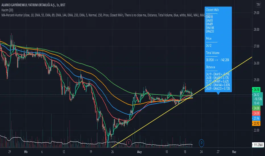
Anticipated Simple Moving Average Crossover IndicatorIntroducing the Anticipated Simple Moving Average Crossover Indicator
This is my Pinescript implementation of the Anticipated Simple Moving Average Crossover Indicator
Much respect to the original creator of this idea Dimitris Tsokakis
This indicator removes one bar of lag from simple moving average crossover signals with a high degree of accuracy to give a slight but very real edge.
Moving Averages
A moving average simplifies price data by smoothing it out by averaging closing prices and creating one flowing line which makes seeing the trend easier.
Moving averages can work well in strong trending conditions, but poorly in choppy or ranging conditions.
Adjusting the time frame can remedy this problem temporarily, although at some point, these issues are likely to occur regardless of the time frame chosen for the moving average(s).
While Exponential moving averages react quicker to price changes than simple moving averages. In some cases, this may be good, and in others, it may cause false signals.
Moving averages with a shorter look back period (20 days, for example) will also respond quicker to price changes than an average with a longer look back period (200 days).
Trading Strategies — Moving Average Crossovers
Moving average crossovers are a popular strategy for both entries and exits. MAs can also highlight areas of potential support or resistance.
The first type is a price crossover, which is when the price crosses above or below a moving average to signal a potential change in trend.
Another strategy is to apply two moving averages to a chart: one longer and one shorter.
When the shorter-term MA crosses above the longer-term MA, it's a buy signal, as it indicates that the trend is shifting up. This is known as a "golden cross."
Meanwhile, when the shorter-term MA crosses below the longer-term MA, it's a sell signal, as it indicates that the trend is shifting down. This is known as a "dead/death cross."
MA and MA Cross Strategy Disadvantages
Moving averages are calculated based on historical data, and while this may appear predictive nothing about the calculation is predictive in nature.
Moving averages are always based on historical data and simply show the average price over a certain time period.
Therefore, results using moving averages can be quite random.
At times, the market seems to respect MA support/resistance and trade signals, and at other times, it shows these indicators no respect.
One major problem is that, if the price action becomes choppy, the price may swing back and forth, generating multiple trend reversal or trade signals.
When this occurs, it's best to step aside or utilize another indicator to help clarify the trend.
The same thing can occur with MA crossovers when the MAs get "tangled up" for a period of time during periods of consolidation, triggering multiple losing trades.
Ensure you use a robust risk management system to avoid getting "Chopped Up" or "Whip Sawed" during these periods.
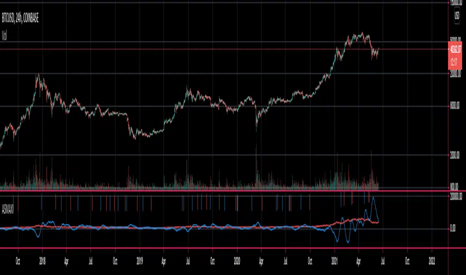
SMA Directional Matrix [LuxAlgo]This script was created in collaboration with alexgrover and displays a simple & elegant panel showing the direction of simple moving averages with periods in a user-selected range (Min, Max). The displayed number in the panel is the period of a simple moving average and the symbol situated at the right of it is associated with the direction this moving average is taking.
Settings
Min: Minimum period of the moving average
Max: Maximum period of the moving average
Src: Source input of the moving averages
Number Of Columns: Number of columns to be displayed in the panel, handy when using a large range of periods.
Usage
Looking at the direction of moving averages with different periods is extremely useful when it comes to having information about the short/mid/long term overall market sentiment, and can also tell us if the market is trending or ranging.
Here we use periods ranging from 25 to 50, we can see that shorter moving averages react to the recent upward price variation, longer-term moving averages however are still affected by the overall downward variation you can see on the image. We can as such get information about the presence of potentials divergences, with shorter-term moving averages reacting to the divergence while the longer-term moving averages will still display the direction of the main trend.
As such the indicator can give information about how clean a trend is, with a clean trend being defined as a variation containing no retracements. When our trend contains no retracement, the mid/long term moving averages will all have the same direction, however, when a retracement is present, the midterm moving averages might be affected by it, thus displaying a direction contrary to the main trend.
When the market is ranging we can expect the panel to display an equal number of decreasing/increasing moving averages.
Possible Issues
When using a large range of periods, you might have an error message showing: "String is too long", try lowering the range of periods by increasing Min or decreasing Max .
If the script displays the error message "Loop is too long to execute", try resetting the settings and change them back to the one you wanted to use.

RSI+ by WilsonThis is a modified version of my RSI Cloud indicator. You can plot 2 moving averages over RSI. You have the option to plot moving average types like SMA, EMA, WMA, VWMA, HullMA, and ALMA. You also have the option to plot histograms based on any of the moving averages. You can fill colors between RSI and moving averages. Option to add alerts, crossover and crossunder signals are also included. I have also included a band to show the position of RSI using three colors. Green color is shown when RSI is above both the plotted moving averages. Red color is shown when RSI is below both the plotted moving averages. And Yellow color is shown when RSI is between the two plotted moving averages. Anyone is free to use the script. Wishing everyone happy and profitable trading.

EMA + SMA - R.AR.A. Trader - Multi-MA Suite (EMA & SMA)
1. Overview
Welcome, students of R.A. Trader!
This indicator is a powerful and versatile tool designed specifically to support the trading methodologies taught by Rudá Alves. The R.A. Trader Multi-MA Suite combines two fully customizable groups of moving averages into a single, clean indicator.
Its purpose is to eliminate chart clutter and provide a clear, at-a-glance view of market trends, momentum, and dynamic levels of support and resistance across multiple timeframes. By integrating key short-term and long-term moving averages, this tool will help you apply the R.A. Trader analytical framework with greater efficiency and precision.
2. Core Features
Dual Moving Average Groups: Configure two independent sets of moving averages, perfect for separating short-term (EMA) and long-term (SMA) analysis.
Four MAs Per Group: Each group contains four fully customizable moving averages.
Multiple MA Types: Choose between several types of moving averages for each group (SMA, EMA, WMA, HMA, RMA).
Toggle Visibility: Easily show or hide each group with a single click in the settings panel.
Custom Styling: Key moving averages are styled for instant recognition, including thicker lines for longer periods and a special dotted line for the 250-period SMA.
Clean and Efficient: The code is lightweight and optimized to run smoothly on the TradingView platform.
Group 1 (Default: EMAs)
This group is pre-configured for shorter-term Exponential Moving Averages but is fully customizable.
Setting Label Description
MA Type - EMA Select the type of moving average for this entire group (e.g., EMA, SMA).
EMA 5 Sets the period for the first moving average.
EMA 10 Sets the period for the second moving average.
EMA 20 Sets the period for the third moving average.
EMA 400 Sets the period for the fourth moving average.
Show EMA Group A checkbox to show or hide all MAs in this group.
Exportar para as Planilhas
Group 2 (Default: SMAs)
This group is pre-configured for longer-term Simple Moving Averages, often used to identify major trends.
Setting Label Description
MA Type - SMA Select the type of moving average for this entire group.
SMA 50 Sets the period for the first moving average.
SMA 100 Sets the period for the second moving average.
SMA 200 Sets the period for the third moving average.
SMA 250 Sets the period for the fourth moving average (styled as a dotted line).
Show SMA Group A checkbox to show or hide all MAs in this group.
Exportar para as Planilhas
Trend TraderDescription and Usage of the "Trend Trader" Indicator
The "Trend Trader" indicator, created by Gerardo Mercado as a legacy project, is a versatile trading tool designed to identify potential buy and sell signals across various instruments. While it provides predefined settings for popular instruments like US30, NDX100, GER40, and GOLD, it can be seamlessly adapted to any market, including forex pairs like EUR/USD. The indicator combines moving averages, time-based filters, and MACD confirmation to enhance decision-making for traders.
How It Works
Custom Moving Averages (MAs):
The indicator uses two moving averages:
Short MA: A faster-moving average (default: 10 periods).
Long MA: A slower-moving average (default: 100 periods).
Buy signals are generated when the Short MA crosses above the Long MA.
Sell signals are triggered when the Short MA crosses below the Long MA.
Time-Based Signals:
The user can define specific trading session times (start and end in UTC) to focus on high-activity periods for their chosen market.
Signals and background coloring are only active during the allowed session times.
MACD Confirmation:
A MACD (Moving Average Convergence Divergence) calculation on a 15-minute timeframe ensures stronger confirmation for signals.
Buy signals require the MACD line to be above the signal line.
Sell signals require the MACD line to be at or below the signal line.
Target Levels:
Predefined profit targets are dynamically set based on the selected trading instrument.
While it includes settings for US30, NDX100, GER40, and GOLD, the target levels can be adjusted to fit the volatility and structure of any asset, including forex pairs like EUR/USD.
Target 1 and Target 2 levels display when these thresholds are met after an entry signal.
Adaptability to Any Market:
Although predefined options are included for specific instruments, the indicator's moving averages, time settings, and MACD logic are applicable to any tradable asset, making it suitable for forex, commodities, indices, and more.
Visual Alerts:
Labels appear on the chart to highlight "BUY" and "SELL" signals at crossover points.
Additional labels indicate when price movements reach the predefined target levels.
Bar and background coloring visually represent active signals and MACD alignment.
Purpose
The indicator aims to simplify trend-following and momentum-based trading strategies. By integrating moving averages, MACD, customizable time sessions, and dynamic targets, it offers clear entry and exit points while being adaptable to the needs of individual traders across diverse markets.
How to Use
Setup:
Add the indicator to your TradingView chart.
Configure the moving average periods, trading session times, and target levels according to your preferences.
Select the instrument for predefined target settings or customize them to fit the asset you’re trading (e.g., EUR/USD or other forex pairs).
Interpreting Signals:
Buy Signal: The Short MA crosses above the Long MA, MACD confirms the upward trend, and the session is active.
Sell Signal: The Short MA crosses below the Long MA, MACD confirms the downward trend, and the session is active.
Adapt for Any Instrument:
Adjust the predefined target levels to match the volatility and trading style for your chosen asset.
For forex pairs like EUR/USD, consider typical pip movements to set appropriate profit targets.
Targets:
Use the provided target labels (e.g., 50 or 100 points) or customize them to reflect realistic profit goals based on the asset’s volatility.
Visual Aids:
Pay attention to the background color:
Greenish: Indicates a bullish trend during the allowed session.
Redish: Indicates a bearish trend during the allowed session.
Use the "BUY" and "SELL" labels for actionable insights.
This indicator is a flexible and powerful tool, suitable for traders across all markets. Its adaptability ensures that it can enhance your strategy, whether you’re trading forex, commodities, indices, or other assets. By offering actionable alerts and customizable settings, the "Trend Trader" serves as a valuable addition to any trader’s toolkit. FX:EURUSD
Heikin-Ashi Mean Reversion Oscillator [Alpha Extract]The Heikin-Ashi Mean Reversion Oscillator combines the smoothing characteristics of Heikin-Ashi candlesticks with mean reversion analysis to create a powerful momentum oscillator. This indicator applies Heikin-Ashi transformation twice - first to price data and then to the oscillator itself - resulting in smoother signals while maintaining sensitivity to trend changes and potential reversal points.
🔶 CALCULATION
Heikin-Ashi Transformation: Converts regular OHLC data to smoothed Heikin-Ashi values
Component Analysis: Calculates trend strength, body deviation, and price deviation from mean
Oscillator Construction: Combines components with weighted formula (40% trend strength, 30% body deviation, 30% price deviation)
Double Smoothing: Applies EMA smoothing and second Heikin-Ashi transformation to oscillator values
Signal Generation: Identifies trend changes and crossover points with overbought/oversold levels
Formula:
HA Close = (Open + High + Low + Close) / 4
HA Open = (Previous HA Open + Previous HA Close) / 2
Trend Strength = Normalized consecutive HA candle direction
Body Deviation = (HA Body - Mean Body) / Mean Body * 100
Price Deviation = ((HA Close - Price Mean) / Price Mean * 100) / Standard Deviation * 25
Raw Oscillator = (Trend Strength * 0.4) + (Body Deviation * 0.3) + (Price Deviation * 0.3)
Final Oscillator = 50 + (EMA(Raw Oscillator) / 2)
🔶 DETAILS Visual Features:
Heikin-Ashi Candlesticks: Smoothed oscillator representation using HA transformation with vibrant teal/red coloring
Overbought/Oversold Zones: Horizontal lines at customizable levels (default 70/30) with background highlighting in extreme zones
Moving Averages: Optional fast and slow EMA overlays for additional trend confirmation
Signal Dashboard: Real-time table showing current oscillator status (Overbought/Oversold/Bullish/Bearish) and buy/sell signals
Reference Lines: Middle line at 50 (neutral), with 0 and 100 boundaries for range visualization
Interpretation:
Above 70: Overbought conditions, potential selling opportunity
Below 30: Oversold conditions, potential buying opportunity
Bullish HA Candles: Green/teal candles indicate upward momentum
Bearish HA Candles: Red candles indicate downward momentum
MA Crossovers: Fast EMA above slow EMA suggests bullish momentum, below suggests bearish momentum
Zone Exits: Price moving out of extreme zones (above 70 or below 30) often signals trend continuation
🔶 EXAMPLES
Mean Reversion Signals: When the oscillator reaches extreme levels (above 70 or below 30), it identifies potential reversal points where price may revert to the mean.
Example: Oscillator reaching 80+ levels during strong uptrends often precedes short-term pullbacks, providing profit-taking opportunities.
Trend Change Detection: The double Heikin-Ashi smoothing helps identify genuine trend changes while filtering out market noise.
Example: When oscillator HA candles change from red to teal after oversold readings, this confirms potential trend reversal from bearish to bullish.
Moving Average Confirmation: Fast and slow EMA crossovers on the oscillator provide additional confirmation of momentum shifts.
Example: Fast EMA crossing above slow EMA while oscillator is rising from oversold levels provides strong bullish confirmation signal.
Dashboard Signal Integration: The real-time dashboard combines oscillator status with directional signals for quick decision-making.
Example: Dashboard showing "Oversold" status with "BUY" signal when HA candles turn bullish provides clear entry timing.
🔶 SETTINGS
Customization Options:
Calculation: Oscillator period (default 14), smoothing factor (1-50, default 2)
Levels: Overbought threshold (50-100, default 70), oversold threshold (0-50, default 30)
Moving Averages: Toggle display, fast EMA length (default 9), slow EMA length (default 21)
Visual Enhancements: Show/hide signal dashboard, customizable table position
Alert Conditions: Oversold bounce, overbought reversal, bullish/bearish MA crossovers
The Heikin-Ashi Mean Reversion Oscillator provides traders with a sophisticated momentum tool that combines the smoothing benefits of Heikin-Ashi analysis with mean reversion principles. The double transformation process creates cleaner signals while the integrated dashboard and multiple confirmation methods help traders identify high-probability entry and exit points during both trending and ranging market conditions.
Clock&Flow MM+InfoThis script is an indicator that helps you visualize various moving averages directly on the price chart and gain some additional insights.
Here's what it essentially does:
Displays Different Moving Averages: You can choose to see groups of moving averages with different periods, set to nominal cyclical durations. You can also opt to configure them for instruments traded with classic or extended trading hours (great for Futures), and they'll adapt to your chosen timeframe.
Colored Bands: It allows you to add colored bands to the background of the chart that change weekly or daily, helping you visualize time cycles. You can customize the band colors.
Information Table: A small table appears in a corner of the chart, indicating which cycle the moving averages belong to (daily, weekly, monthly, etc.), corresponding to the timeframe you are using on the chart.
Customization: You can easily enable or disable the various groups of moving averages or the colored bands through the indicator's settings.
It's a useful tool for traders who use moving averages to identify trends and support/resistance levels, and who want a quick overview of market cycles.
Questo script è un indicatore che aiuta a visualizzare diverse medie mobili direttamente sul grafico dei prezzi e a ottenere alcune informazioni aggiuntive.
In pratica, fa queste cose:
Mostra diverse medie mobili: Puoi scegliere di vedere gruppi di medie mobili con periodi diversi impostati sulle durate cicliche nominali. Puoi scegliere se impostarle per uno strumento quotato con orario di negoziazione classico o esteso (ottimo per i Futures) e si adattano al tuo timeframe).
Bande colorate: Ti permette di aggiungere delle bande colorate sullo sfondo del grafico che cambiano ogni settimana o ogni giorno, per aiutarti a visualizzare i cicli temporali. Puoi scegliere il colore delle bande.
Tabella informativa: In un angolo del grafico, compare una piccola tabella che indica a quale ciclo appartengono le medie mobili (giornaliero, settimanale, mensile, ecc.) e corrispondono in base al timeframe che stai usando sul grafico.
Personalizzazione: Puoi facilmente attivare o disattivare i vari gruppi di medie mobili o le bande colorate tramite le impostazioni dell'indicatore.
È uno strumento utile per i trader che usano le medie mobili per identificare trend e supporti/resistenze, e che vogliono avere un colpo d'occhio sui cicli di mercato.
Price Flip StrategyPrice Flip Strategy with User-Defined Ticker Max/Max
This strategy leverages an inverted price calculation based on user-defined maximum and minimum price levels over customizable lookback periods. It generates buy and sell signals by comparing the previous bar's original price to the inverted price, within a specified date range. The script plots key metrics, including ticker max/min, original and inverted prices, moving averages, and HLCC4 averages, with customizable visibility toggles and labels for easy analysis.
Key Features:
Customizable Inputs: Set lookback periods for ticker max/min, moving average length, and date range for signal generation.
Inverted Price Logic: Calculates an inverted price using ticker max/min to identify trading opportunities.
Flexible Visualization: Toggle visibility for plots (e.g., ticker max/min, prices, moving averages, HLCC4 averages) and last-bar labels with user-defined colors and sizes.
Trading Signals: Generates buy signals when the previous original price exceeds the inverted price, and sell signals when it falls below, with alerts for real-time notifications.
Labeling: Displays values on the last bar for all plotted metrics, aiding in quick reference.
How to Use:
Add to Chart: Apply the script to a TradingView chart via the Pine Editor.
Configure Settings:
Date Range: Set the start and end dates to define the active trading period.
Ticker Levels: Adjust the lookback periods for calculating ticker max and min (e.g., 100 bars for max, 100 for min).
Moving Averages: Set the length for exponential moving averages (default: 20 bars).
Plots and Labels: Enable/disable specific plots (e.g., Inverted Price, Original HLCC4) and customize label colors/sizes for clarity.
Interpret Signals:
Buy Signal: Triggered when the previous close price is above the inverted price; marked with an upward label.
Sell Signal: Triggered when the previous close price is below the inverted price; marked with a downward label.
Set Alerts: Use the built-in alert conditions to receive notifications for buy/sell signals.
Analyze Plots: Review plotted lines (e.g., ticker max/min, HLCC4 averages) and last-bar labels to assess price behavior.
Tips:
Use in trending markets by enabling ticker max for uptrends or ticker min for downtrends, as indicated in tooltips.
Adjust the label offset to prevent overlapping text on the last bar.
Test the strategy on a demo account to optimize lookback periods and moving average settings for your asset.
Disclaimer: This script is for educational purposes and should be tested thoroughly before use in live trading. Past performance is not indicative of future results.
Displaced MAsDisplaced Moving Averages with Customizable Bands
Overview
The "Displaced Moving Averages with Customizable Bands" indicator is a powerful and versatile tool designed to provide a comprehensive view of price action in relation to various moving averages (MAs) and their volatility. It offers a high degree of customization, allowing traders to tailor the indicator to their specific needs and trading styles. The indicator features a primary moving average with multiple configurable percentage-based displacement bands. It also includes additional moving averages with standard deviation bands for a more in-depth analysis of different timeframes.
Key Features
Multiple Moving Average Types:
Choose from a wide range of popular moving average types for the primary MA calculation:
WMA (Weighted Moving Average)
EMA (Exponential Moving Average)
SMA (Simple Moving Average)
HMA (Hull Moving Average)
VWAP (Volume-Weighted Average Price)
Smoothed VWAP
Rolling VWAP
The flexibility to select the most appropriate MA type allows you to adapt the indicator to different market conditions and trading strategies.
Smoothed VWAP with Customizable Smoothing:
When "Smoothed VWAP" is selected, you can further refine it by choosing a smoothing type: SMA, EMA, WMA, or HMA.
Customize the smoothing period based on the chart's timeframe (1H, 4H, D, W) or use a default period. This feature offers fine-grained control over the responsiveness of the VWAP calculation.
Rolling VWAP with Adjustable Lookback:
The "Rolling VWAP" option calculates the VWAP over a user-defined lookback period.
Customize the lookback length for different timeframes (1H, 4H, D, W) or use a default period. This provides a dynamic VWAP calculation that adapts to the chosen timeframe.
Customizable Lookback Lengths:
Define the lookback period for the primary moving average calculation.
Tailor the lookback lengths for different timeframes (1H, 4H, D, W) or use a default value.
This allows you to adjust the sensitivity of the MA to recent price action based on the timeframe you are analyzing. Also has inputs for 5m, and 15m timeframes.
Percentage-Based Displacement Bands:
The core feature of this indicator is the ability to plot multiple displacement bands above and below the primary moving average.
These bands are calculated as a percentage offset from the MA, providing a clear visualization of price deviations.
Visibility Toggles: Independently show or hide each band (+/- 2%, 5%, 7%, 10%, 15%, 20%, 25%, 30%, 40%, 50%, 60%, 70%).
Customizable Colors: Assign unique colors to each band for easy visual identification.
Adjustable Multipliers: Fine-tune the percentage displacement for each band using individual multiplier inputs.
The bands are useful for identifying potential support and resistance levels, overbought/oversold conditions, and volatility expansions/contractions.
Labels for Displacement Bands:
The indicator displays labels next to each plotted band, clearly indicating the percentage displacement (e.g., "+7%", "-15%").
Customize the label text color for optimal visibility.
The labels can be horizontally offset by a user-defined number of bars.
Additional Moving Averages with Standard Deviation Bands:
The indicator includes three additional moving averages, each with upper and lower standard deviation bands. These are designed to provide insights into volatility on different timeframes.
Timeframe Selection: Choose the timeframes for these additional MAs (e.g., Weekly, 4-Hour, Daily).
Sigma (Standard Deviation Multiplier): Adjust the standard deviation multiplier for each MA.
MA Length: Set the lookback period for each additional MA.
Visibility Toggles: Show or hide the lower band of MA1, the middle/upper/lower bands of MA2, and the bands of MA3.
4h Bollinger Middle MA is unticked by default to provide a less cluttered chart
These additional MAs are particularly useful for multi-timeframe analysis and identifying potential trend reversals or volatility shifts.
How to Use
Add the indicator to your TradingView chart.
Customize the settings:
Select the desired Moving Average Type for the primary MA.
If using Smoothed VWAP, choose the Smoothing Type and adjust the Smoothing Period for different timeframes.
If using Rolling VWAP, adjust the Lookback Length for different timeframes.
Set the Lookback Length for the primary MA for different timeframes.
Toggle the visibility of the Displacement Bands and adjust their Colors and Multipliers.
Customize the Label Text Color and Offset.
Configure the Timeframes, Sigma, and MA Length for the additional moving averages.
Toggle the visibility of the additional MA bands.
Interpret the plotted lines and bands:
Primary MA: Represents the average price over the selected lookback period, calculated using the chosen MA type.
Displacement Bands: Indicate potential support and resistance levels, overbought/oversold conditions, and volatility ranges. Price trading outside these bands may signal significant deviations from the average.
Additional MAs with Standard Deviation Bands: Provide insights into volatility on different timeframes. Wider bands suggest higher volatility, while narrower bands indicate lower volatility.
Potential Trading Applications
Trend Identification: Use the primary MA to identify the overall trend direction.
Support and Resistance: The displacement bands can act as dynamic support and resistance levels.
Overbought/Oversold: Price reaching the outer displacement bands may suggest overbought or oversold conditions, potentially indicating a pullback or reversal.
Volatility Analysis: The standard deviation bands of the additional MAs can help assess volatility on different timeframes.
Multi-Timeframe Analysis: Combine the primary MA with the additional MAs to gain a broader perspective on price action across multiple timeframes.
Entry and Exit Signals: Use the interaction of price with the MA and bands to generate potential entry and exit signals. For example, a bounce off a lower band could be a buy signal, while a rejection from an upper band could be a sell signal.
Disclaimer
This indicator is for informational and educational purposes only and should not be considered financial advice. Trading involves risk, and past performance is not indicative of future results. Always conduct thorough research and consider your risk tolerance before making any trading decisions.
Enjoy using the "Displaced Moving Averages with Customizable Bands" indicator!

Adaptive Fibonacci Trend Ribbon[FibonacciFlux]Adaptive Fibonacci Trend Ribbon (FibonacciFlux)
Overview
The Adaptive Fibonacci Trend Ribbon is a versatile technical analysis tool designed for traders who want to leverage the power of multiple moving averages while integrating Fibonacci numbers. This indicator provides a dynamic visual representation of market trends, enhancing decision-making processes in trading.
Key Features
1. Multi-Moving Averages
- The indicator calculates eight different moving averages based on user-defined periods, including Fibonacci numbers such as 5, 8, 13, 21, 34, 55, 89, and 144.
- Traders can choose from various moving average types, including EMA, HMA, WMA, VWMA, ALMA, SMA, RMA, and TMA , allowing for tailored analysis based on market conditions.
2. Trend Detection
- Each moving average is color-coded based on its trend direction, with green indicating an upward trend and red indicating a downward trend.
- This visual clarity helps traders quickly assess market sentiment and make informed decisions.
3. Fill Areas for Enhanced Insight
- The indicator features fill areas between the moving averages, which dynamically change color according to their relative positions.
- This provides a clear visual cue of trend strength and potential reversal points, allowing traders to identify key areas of interest.
4. Customizable Inputs
- Users can easily adjust the source data, moving average lengths, and ALMA parameters (offset and sigma) to fit their trading strategies.
- This flexibility ensures that traders can adapt the tool to various market conditions and personal preferences.
Insights and Applications
1. Fibonacci Integration
- By incorporating Fibonacci numbers into the moving average periods, this indicator allows traders to align their strategies with key levels of support and resistance.
- This can enhance the accuracy of entry and exit points, particularly in trending markets.
2. Trend Continuation and Reversal Analysis
- The adaptive nature of the moving averages provides insights into potential trend continuations or reversals.
- Traders can use the indicator to identify when to enter or exit positions based on the interaction between the moving averages.
3. Visual Clarity for Quick Decisions
- The color-coded moving averages and fill areas offer immediate visual feedback on market conditions, helping traders react swiftly to changing dynamics.
- This is especially useful in fast-moving markets where timely decisions are critical.
Conclusion
The Adaptive Fibonacci Trend Ribbon is an essential tool for traders looking to enhance their technical analysis capabilities. By combining multiple moving averages with Fibonacci integration and dynamic visual cues, this indicator offers a robust framework for understanding market trends. Its flexibility and clarity make it an invaluable asset for both novice and experienced traders alike.
Open Source Contribution
This indicator is open source, inviting contributions and improvements from the trading community. Feel free to fork, enhance, and share your insights with the world, helping to foster a collaborative environment for traders everywhere.