Swiss Knife [MERT]Introduction
The Swiss Knife indicator is a comprehensive trading tool designed to provide a multi-dimensional analysis of the market. By integrating a wide array of technical indicators across multiple timeframes, it offers traders a holistic view of market sentiment, momentum, and potential reversal points. This indicator is particularly useful for traders looking to combine trend analysis, momentum indicators, volume data, and price action into a single, easy-to-read format.
---
Key Features
Multi-Timeframe Analysis : Evaluates indicators on Daily , 4-Hour , 1-Hour , and 15-Minute timeframes.
Comprehensive Indicator Suite : Incorporates MACD , Awesome Oscillator (AO) , Parabolic SAR , SuperTrend , DPO , RSI , Stochastic Oscillator , Bollinger Bands , Ichimoku Cloud , Chande Momentum Oscillator (CMO) , Donchian Channels , ADX , volume-based momentum indicators, Fractals , and divergence detection.
Market Sentiment Scoring : Aggregates signals from multiple indicators to provide an overall sentiment score.
Visual Aids : Displays EMA lines, trendlines, divergence signals, and a sentiment table directly on the chart.
Super Trend Reversal Signals : Identifies potential market reversal points by assessing the momentum of automated trading bots.
---
Explanation of Each Indicator
Moving Average Convergence Divergence (MACD)
- Purpose : Measures the relationship between two moving averages of price.
- Interpretation : A positive histogram suggests bullish momentum; a negative histogram indicates bearish momentum.
Awesome Oscillator (AO)
- Purpose : Gauges market momentum by comparing recent market movements to historic ones.
- Interpretation : Above zero indicates bullish momentum; below zero indicates bearish momentum.
Parabolic SAR (SAR)
- Purpose : Identifies potential reversal points in price direction.
- Interpretation : Dots below price suggest an uptrend; dots above price suggest a downtrend.
SuperTrend
- Purpose : Determines the prevailing market trend.
- Interpretation : Provides buy or sell signals based on price movements relative to the SuperTrend line.
Detrended Price Oscillator (DPO)
- Purpose : Removes trend from price to identify cycles.
- Interpretation : Values above zero suggest price is above the moving average; values below zero indicate it is below.
Relative Strength Index (RSI)
- Purpose : Measures the speed and change of price movements.
- Interpretation : Values above 50 indicate bullish momentum; values below 50 indicate bearish momentum.
Stochastic Oscillator
- Purpose : Compares a particular closing price to a range of its prices over a certain period.
- Interpretation : Values above 50 indicate bullish conditions; values below 50 indicate bearish conditions.
Bollinger Bands (BB)
- Purpose : Measures market volatility and provides relative price levels.
- Interpretation : Price above the middle band suggests bullishness; below the middle band suggests bearishness.
Ichimoku Cloud
- Purpose : Provides support and resistance levels, trend direction, and momentum.
- Interpretation : Bullish signals when price is above the cloud; bearish signals when price is below the cloud.
Chande Momentum Oscillator (CMO)
- Purpose : Measures momentum on both up and down days.
- Interpretation : Values above 50 indicate strong upward momentum; values below -50 indicate strong downward momentum.
Donchian Channels
- Purpose : Identifies volatility and potential breakouts.
- Interpretation : Price above the upper band suggests bullish breakout; below the lower band suggests bearish breakout.
Average Directional Index (ADX)
- Purpose : Measures the strength of a trend.
- Interpretation : DI+ above DI- indicates bullish trend; DI- above DI+ indicates bearish trend.
Volume Momentum Indicators (VolMom, CumVolMom, POCMom)
- Purpose : Analyze volume to assess buying and selling pressure.
- Interpretation : Positive values suggest bullish volume momentum; negative values indicate bearish volume momentum.
Fractals
- Purpose : Identify potential reversal points in the market.
- Interpretation : Up fractals may indicate a future downtrend; down fractals may indicate a future uptrend.
Divergence Detection
- Purpose : Identifies divergences between price and various indicators (RSI, MACD, Stochastic, OBV, MFI, A/D Line).
- Interpretation : Bullish divergences suggest potential upward reversal; bearish divergences suggest potential downward reversal.
- Note : This functionality utilizes the library from Divergence Indicator .
---
Coloring Scheme
Background Color
- Purpose : Reflects the overall market sentiment by combining sentiment scores from all indicators across different timeframes.
- Interpretation :
- Green Shades : Indicate bullish market sentiment.
- Red Shades : Indicate bearish market sentiment.
- Intensity : The strength of the color corresponds to the strength of the sentiment score.
Sentiment Table
- Purpose : Displays the status of each indicator across different timeframes.
- Interpretation :
- Green Cell : The indicator suggests a bullish signal.
- Red Cell : The indicator suggests a bearish signal.
- Percentage Score : Indicates the overall bullish or bearish sentiment on that timeframe.
Exponential Moving Averages (EMAs)
- Purpose : Provide dynamic support and resistance levels.
- Colors :
- EMA 10 : Lime
- EMA 20 : Yellow
- EMA 50 : Orange
- EMA 100 : Red
- EMA 200 : Purple
Trendlines
- Purpose : Visual representation of support and resistance levels based on pivot points.
- Interpretation :
- Upward Trendlines : Colored green , indicating support levels.
- Downward Trendlines : Colored red , indicating resistance levels.
- Note : Trendlines are drawn using the library from Simple Trendlines .
---
Utility of Market Sentiment
The indicator aggregates signals from multiple technical indicators across various timeframes to compute an overall market sentiment score . This comprehensive approach helps traders understand the prevailing market conditions by:
Confirming Trends : Multiple indicators pointing in the same direction can confirm the strength of a trend.
Identifying Reversals : Divergences and fractals can signal potential turning points.
Timeframe Alignment : Aligning signals across different timeframes can enhance the probability of successful trades.
---
Divergences
Divergence occurs when the price of an asset moves in the opposite direction of a technical indicator, suggesting a potential reversal.
- Bullish Divergence : Price makes a lower low, but the indicator makes a higher low.
- Bearish Divergence : Price makes a higher high, but the indicator makes a lower high.
The indicator detects divergences for:
RSI
MACD
Stochastic Oscillator
On-Balance Volume (OBV)
Money Flow Index (MFI)
Accumulation/Distribution Line (A/D Line)
By identifying these divergences, traders can spot early signs of trend reversals and adjust their strategies accordingly.
---
Trendlines
Trendlines are essential tools for identifying support and resistance levels. The indicator automatically draws trendlines based on pivot points:
- Upward Trendlines (Support) : Connect higher lows, indicating an uptrend.
- Downward Trendlines (Resistance) : Connect lower highs, indicating a downtrend.
These trendlines help traders visualize the trend direction and potential breakout or reversal points.
---
Super Trend Reversals (ST Reversal)
The core idea behind the Super Trend Reversals indicator is to assess the momentum of automated trading bots (often referred to as 'Supertrend bots') that enter the market during critical turning points. Specifically, the indicator is tuned to identify when the market is nearing bottoms or peaks, just before it shifts direction based on the triggered Supertrend signals. This approach helps traders:
Engage Early : Enter the market as reversal momentum builds up.
Optimize Entries and Exits : Enter under favorable conditions and exit before momentum wanes.
By capturing these reversal points, traders can enhance their trading performance.
---
Conclusion
The Swiss Knife indicator serves as a versatile tool that combines multiple technical analysis methods into a single, comprehensive indicator. By assessing various aspects of the market—including trend direction, momentum, volume, and price action—it provides traders with valuable insights to make informed trading decisions.
---
Citations
- Divergence Detection Library : Divergence Indicator by DevLucem
- Trendline Drawing Library : Simple Trendlines by HoanGhetti
---
Note : This indicator is intended for informational purposes and should be used in conjunction with other analysis techniques. Always perform due diligence before making trading decisions.
---
Buscar en scripts para "bot"

Super Trend ReversalsMain Concept
The core idea behind the Super Trend Reversals indicator is to assess the momentum of automated trading bots (often referred to as 'Supertrend bots') that enter the market during critical turning points. Specifically, the indicator is tuned to identify when the market is nearing bottoms or peaks, but just before it shifts direction based on the triggered Supertrend signals. This approach helps traders engage with the market right as the reversal momentum builds up, allowing for entry just as conditions become favorable and exit before momentum wanes.
How It Works
The Super Trend Reversals uses multiple Supertrend calculations, each with different period and multiplier settings, to form a comprehensive view of the trend. The total trend score from these calculations is then analyzed using the Relative Strength Index (RSI) and Exponential Moving Averages (EMA) to gauge the strength and sustainability of the trend.
A key feature of this indicator is the isCurrentRangeSmaller() function, which evaluates if the current price range is lower than the average over the recent period. This function is critical as it helps determine the stability of the market environment, reducing the likelihood of entering or exiting trades based on erratic price movements that could lead to false signals.

speed of tradesThis indicator calculates the speed of trades, on other platform that is called speed of tape, but they said you need delta and others for the calculation.
Calculation method
This indicator calculates the number of trades per bar and filter it, if they are above a sma it highlights the column to know that could be a bar where there are more trades than usual.
It's based on an example of pinescript v5 user manual where explain the use of varip
HF Bots filter and common uses
know where there are more trades than usual help you to have an idea that could be HF Bots working on that bar, also if you dont belive on that, can also help you to have an idea of momentum or stoping action.
Why is this indicator original?
The speed of trades indicator give you an counter of number of trades and a filter for bars where there are a lot of trades, so searching speed of tape/trades indicator that don't exist on tradingview, this indicator is original.
How to charge data?
By default it doesn't load historical tick data, this indicator only works on realtime bars.

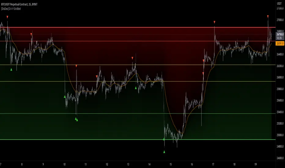
[DisDev] D-I-Y Gridbot🟩 This script is a “do-it-yourself” Grid Bot Simulator, used for visualizing support and resistance levels. Prices are divided into grids, or trade zones, that will trigger signals each time a new zone is entered. During ranging markets, each transaction is followed by a “take profit.” As the market starts to trend, transactions are stacked (compare to DCA ), until the market consolidates. No signals are triggered above the upper gridline or below the lower gridline. Unlike the previous version, all grids may be adjusted in real-time by dragging the gridlines up and down to the desired support and resistance levels.
When adding the indicator to a new chart, you must choose six grid levels by clicking on the desired support or resistance price. You can change all of these levels at any time directly on the chart.
⚡ OVERVIEW ⚡
The D-I-Y Gridbot is an interactive tool designed for visualizing support and resistance levels. As a continuation of the original Gridbot Simulator , which has received significant recognition on TradingView, earning over 4000 boosts and an Editor's Pick status. This tool serves not only as an evolved version of its predecessor, but also as an open-source template for developing future gridbots. It aims to foster discussions and facilitate innovations around grid-trading strategies.
One of the new features of this gridbot is the real-time adjustability of all gridlines. Users can move these lines up and down to set their desired support and resistance levels in response to changing market conditions. Additionally, the D-I-Y Gridbot is compatible with multiple timeframes and can be used on most TradingView charts.
Drag gridlines up or down to desired price level.
Key Features 🔑
All gridlines are adjustable in real-time, directly on the chart
Signals can be filtered by a customizable moving average or by VWAP
Customizable support and resistance levels
Potentially increases profitability in ranging markets
Benefits 💸
Customizable Support and Resistance Levels : The D-I-Y Gridbot allows users to set their preferred support and resistance levels, which can be changed at any time directly on the chart. This provides users with the ability to customize their trading parameters based on their strategy and risk tolerance.
Various Trading Strategies : The D-I-Y Gridbot supports various trading strategies, including Mean Reversion, Ranging Markets, and Dollar-cost averaging (DCA). This allows users to capitalize on price reversals, execute buy and sell orders at predetermined levels, and buy more of an asset as the price falls, respectively.
Multi-Timeframe and Versatility : The D-I-Y Gridbot is compatible with multiple timeframes and can be used on any TradingView chart.
Experimental and Educational : The D-I-Y Gridbot is considered a proof-of-concept tool that is both experimental and educational. This can provide traders with a deeper understanding of grid trading strategies and the ability to experiment with different trading parameters and strategies.
⚙️ CONFIGURATION & SETTINGS ⚙️
Inputs 🔧
Trigger : Candle location to trigger the signal. "Wick" will use either high or low, depending on the signal direction. "Close" will use the close price. “MA” will use the selected moving average or VWAP.
Confirmation : Market direction to confirm the candle trigger. "Reverse" will confirm the signal when the price crosses back over the trigger. "Breakout" will confirm when the price breaks out of the trigger.
Number of Support/Resistance zones : 1 = Only Top Grid is Support/Only Bottom Grid is Resistance. 2 = Top two grids are Resistance/Bottom two grids are Support. 3 = Top three grids are Resistance/Bottom three grids are Support
MA Type : Exponential Moving Average (EMA), Hull Moving Average (HMA), Simple Moving Average (SMA), Triple Exponential Moving Average (TEMA), Volume Weighted Moving Average (VWMA), Volume Weighted Average Price (VWAP)
MA Filter : Use Moving Average as a reversion filter for signals. When enabled, no buys when above MA, no sells when below. Use in conjunction with S/R zones to reduce false signals.
Allow Repeat Signals . When enabled, signals will reset when nearest gridline is triggered. When disabled, only one signal will be triggered per gridline.
Line/Fill colors
Gridlines . Adjusts gridline prices manually.
Left : Trigger = Wick. Confirm = Breakout. Buys are signaled when LOW breaks below gridline. Sells are triggered when HIGH breaks above gridline.
Right : Trigger = Close. Confirm = Breakout. Buys are signaled when the candle CLOSES below the gridline. Sells are triggered when the candle CLOSES above the gridline.
Left : Confirm=Breakout. Signals on breaking through the next gridline.
Right : Confirm=Reverse. Signals only when crossing back from the gridline.
S/R Zones=1. Upper gridline is Resistance / Lower is Support. Middle 4 are neutral.
S/R Zones = 3. Upper three gridlines are Resistance / Lower three are Support
Notes:
If gridlines are dragged out of order on a live chart, they will auto-sort into the correct order.
Price levels may be entered in settings, or adjusted in real-time directly on the chart.
When changing symbols, remember to adjust the gridlines to accommodate the new symbol.
Alerts 🔔
Users can set alerts based on their chosen parameters for triggers, confirmations, number of support/resistance zones, and smoothing type, enabling precise control over alert conditions.
💡 USAGE & STRATEGY 💡
Trading Strategies 📈
Mean Reversion: The script can be used to capitalize on price reversals back to the mean.
Ranging Markets: The script excels in ranging markets, executing buy and sell orders at predetermined levels.
Dollar-cost averaging (DCA): The script can be used to execute DCA orders, buying more of an asset as the price falls, and lowering the average cost per unit.
Timeframes and Symbols ⌚
Multi-Timeframe: The indicator is compatible with multiple timeframes.
Versatile: Can be used on any crypto trading pair on TradingView.
🤖 DETAILS & METHODOLOGY 🤖
Algorithm and Calculation 🛡️
Grids are set and adjusted when loading the indicator on the chart and may be customized anytime afterward by clicking and dragging the gridlines on the chart.
Gridlines are updated, sorted, and stored in a float array.
Signals are calculated based on candle trigger, market direction, and previous price level.
📚 ADDITIONAL RESOURCES 📚
Chart Examples 📊
S/R Zones = 3: Three Support and Three Resistance. Filter = 50-period Triple Exponential Moving Average (TEMA)
S/R Zones = 1: One Support, One Resistance, and Four Neutral Zones. Support Zones: Buys only. Resistance Zones: Sells only. Neutral Zones: Grid-dependent
When MA filter is enabled, Buys are only triggered below Moving Average, and Sells are only triggered above.
Trigger = Wick. Confirmation = Breakout. Buys are signaled when Low breaks above the next grid level. Sells are signaled when High breaks below the next grid level.
🚀 CONCLUSION 🚀
The D-I-Y Gridbot is a proof-of-concept, emphasizing its experimental and educational nature. In future versions, we will aim to incorporate concepts such as auto-adjusting grids and angled grids for trending markets. The script is designed to evolve through user feedback and suggestions, shaping its future iterations.
Credit: This is a continuation of the Gridbot series by xxattaxx-DisDev . Explicit permission was granted by user xxattaxx-disdev to re-use all Gridbot code and all materials without restrictions.
⚠️ DISCLAIMER ⚠️
This indicator is a proof-of-concept and is considered experimental and educational. When gridlines are drawn in hindsight, signals appear to be predictive and valid. Future results may always vary when the trend direction changes. Comments and suggestions are encouraged.
This indicator is provided as a tool for traders and should not be used as the sole basis for making trading decisions. Always conduct your own research and consider your risk tolerance before entering any trades.
Keltner Trend V3It's just a simple keltner trend with options added to:
Eradicate repainting
more MAs
Json alerts (useful for bots)
I recommend using "open" option for all sources if you are going to use it with a bot, or if you want to be safe and enter with confirmations. Using the default settings would also show you all the entries without repainting as it uses high and low prices to check breakouts and not solely the close price (which is generally a false representative in historic analysis).
My favorite lengths are 7, 14, and 21. There is no specific reason, they just seem to work well most of the time. You can (and should) optimize it to your purposes.
Thanks to the original author @jaggedsoft this script is just a improved version of theirs.

Сoncentrated Market Maker Strategy by oxowlConcentrated Market Maker Strategy by oxowl. This script plots an upper and lower bound for liquidity provision, and checks for rebalancing conditions. It also includes alert conditions for when the price crosses the upper or lower bounds.
Here's an overview of the script:
It defines the input parameters: liquidity range percentage, rebalance frequency in minutes, and minimum trade size in assets.
It calculates the upper and lower bounds for liquidity provision based on the liquidity range percentage.
It initializes variables for the last rebalance time and price.
It defines a rebalance condition based on the frequency and current price within the specified range.
If the rebalance condition is met, it updates the last rebalance time and price.
It plots the upper and lower bounds on the chart as lines and adds price labels for both bounds.
It defines alert conditions for when the price crosses the upper or lower bounds.
Finally, it creates alert conditions with appropriate messages for when the price crosses the upper or lower bounds.
Concentrated liquidity is a concept often used in decentralized finance (DeFi) market-making strategies. It allows liquidity providers (LPs) to focus their liquidity within a specific price range, rather than across the entire price curve. Using an indicator with concentrated liquidity can offer several advantages:
Increased capital efficiency: Concentrated liquidity allows LPs to allocate their capital within a narrower price range. This means that the same amount of capital can generate more significant price impact and potentially higher returns compared to providing liquidity across a broader range.
Customized risk exposure: LPs can choose the price range they feel most comfortable with, allowing them to better manage their risk exposure. By selecting a range based on their market outlook, they can optimize their positions to maximize potential returns.
Adaptive strategies: Indicators that support concentrated liquidity can help traders adapt their strategies based on market conditions. For example, they can choose to provide liquidity around a stable price range during low-volatility periods or adjust their range when market conditions change.
To continue integrating this script into your trading strategy, follow these steps:
Import the script into your TradingView account. Navigate to the Pine editor, paste the code, and save it as a new script.
Apply the indicator to a trading pair chart. You can customize the input parameters (liquidity range percentage, rebalance frequency, and minimum trade size) based on your preferences and risk tolerance.
Set alerts for when the price crosses the upper or lower bounds. This will notify you when it's time to take action, such as adding or removing liquidity, or rebalancing your position.
Monitor the performance of your strategy over time. Adjust the input parameters as needed to optimize your returns and manage risk effectively.
(Optional) Integrate the script with a trading bot or automation platform. If you're using an API-based trading solution, you can incorporate the logic and conditions from the script into your bot's algorithm to automate the process of providing concentrated liquidity and rebalancing your positions.
Remember that no strategy is foolproof, and past performance is not indicative of future results. Always exercise caution when trading and carefully consider your risk tolerance.

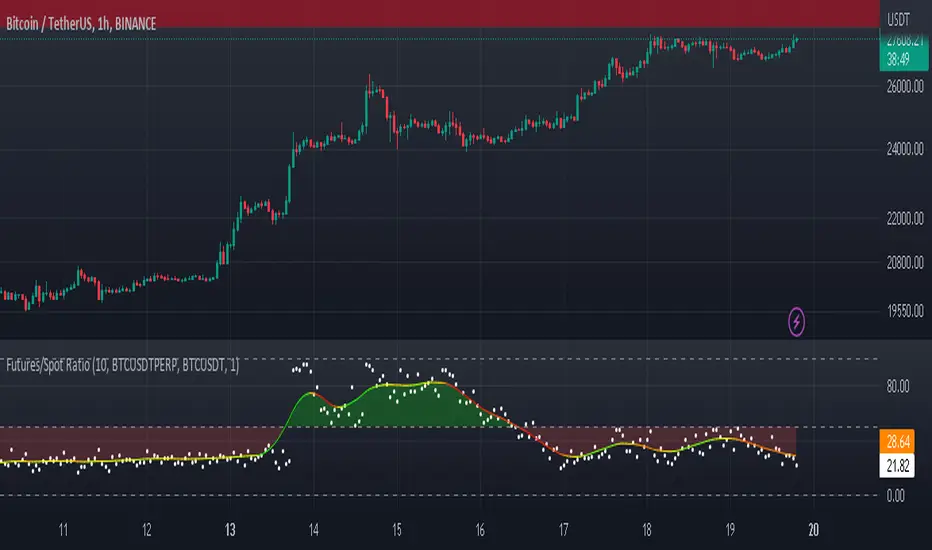
Futures/Spot Ratiowhat is Futures /Spot Ratio?
Although futures and spot markets are separate markets, they are correlated. arbitrage bots allow this gap to be closed. But arbitrage bots also have their limits. so there are always slight differences between futures and spot markets. By analyzing these differences, the movements of the players in the market can be interpreted and important information about the price can be obtained. Futures /Spot Ratio is a tool that facilitates this analysis.
what it does?
it compresses the ratio between two selected spot and futures trading pairs between 0 and 100. its purpose is to facilitate use and interpretation. it also passes a regression (Colorful Regression) through the middle of the data for the same purpose.
about Colorful Regression:
how it does it?
it uses this formula:
how to use it?
use it to understand whether the market is priced with spot trades or leveraged positions. A value of 50 is the breakeven point where the ratio of the spot and leveraged markets are equal. Values above 50 indicate excess of long positions in the market, values below 50 indicate excess of short positions. I have explained how to interpret these ratios with examples below.
Simple_RSI+PA+DCA StrategyThis strategy is a result of a study to understand better the workings of functions, for loops and the use of lines to visualize price levels. The strategy is a complete rewrite of the older RSI+PA+DCA Strategy with the goal to make it dynamic and to simplify the strategy settings to the bare minimum.
In case you are not familiar with the older RSI+PA+DCA Strategy, here is a short explanation of the idea behind the strategy:
The idea behind the strategy based on an RSI strategy of buying low. A position is entered when the RSI and moving average conditions are met. The position is closed when it reaches a specified take profit percentage. As soon as the first the position is opened multiple PA (price average) layers are setup based on a specified percentage of price drop. When the price hits the layer another position with the same position size is is opened. This causes the average cost price (the white line) to decrease. If the price drops more, another position is opened with another price average decrease as result. When the price starts rising again the different positions are separately closed when each reaches the specified take profit. The positions can be re-opened when the price drops again. And so on. When the price rises more and crosses over the average price and reached the specified Stop level (the red line) on top of it, it closes all the positions at once and cancels all orders. From that moment on it waits for another price dip before it opens a new position.
This is the old RSI+PA+DCA Strategy:
The reason to completely rewrite the code for this strategy is to create a more automated, adaptable and dynamic system. The old version is static and because of the linear use of code the amount of DCA levels were fixed to max 6 layers. If you want to add more DCA layers you manually need to change the script and add extra code. The big difference in the new version is that you can specify the amount of DCA layers in the strategy settings. The use of 'for loops' in the code gives the possibility to make this very dynamic and adaptable.
The RSI code is adapted, just like the old version, from the RSI Strategy - Buy The Dips by Coinrule and is used for study purpose. Any other low/dip finding indicator can be used as well
The distance between the DCA layers are calculated exponentially in a function. In the settings you can define the exponential scale to create the distance between the layers. The bigger the scale the bigger the distance. This calculation is not working perfectly yet and needs way more experimentation. Feel free to leave a comment if you have a better idea about this.
The idea behind generating DCA layers with a 'for loop' is inspired by the Backtesting 3commas DCA Bot v2 by rouxam .
The ideas for creating a dynamic position count and for opening and closing different positions separately based on a specified take profit are taken from the Simple_Pyramiding strategy I wrote previously.
This code is a result of a study and not intended for use as a full functioning strategy. To make the code understandable for users that are not so much introduced into pine script (like myself), every step in the code is commented to explain what it does. Hopefully it helps.
Enjoy!

libKageMiscLibrary "libKageMisc"
Kage's Miscelaneous library
print(_value)
Print a numerical value in a label at last historical bar.
Parameters:
_value : (float) The value to be printed.
Returns: Nothing.
barsBackToDate(_year, _month, _day)
Get the number of bars we have to go back to get data from a specific date.
Parameters:
_year : (int) Year of the specific date.
_month : (int) Month of the specific date. Optional. Default = 1.
_day : (int) Day of the specific date. Optional. Default = 1.
Returns: (int) Number of bars to go back until reach the specific date.
bodySize(_index)
Calculates the size of the bar's body.
Parameters:
_index : (simple int) The historical index of the bar. Optional. Default = 0.
Returns: (float) The size of the bar's body in price units.
shadowSize(_direction)
Size of the current bar shadow. Either "top" or "bottom".
Parameters:
_direction : (string) Direction of the desired shadow.
Returns: (float) The size of the chosen bar's shadow in price units.
shadowBodyRatio(_direction)
Proportion of current bar shadow to the bar size
Parameters:
_direction : (string) Direction of the desired shadow.
Returns: (float) Ratio of the shadow size per body size.
bodyCloseRatio(_index)
Proportion of chosen bar body size to the close price
Parameters:
_index : (simple int) The historical index of the bar. Optional. Default = 0.()
Returns: (float) Ratio of the body size per close price.
lastDayOfMonth(_month)
Returns the last day of a month.
Parameters:
_month : (int) Month number.
Returns: (int) The number (28, 30 or 31) of the last day of a given month.
nameOfMonth(_month)
Return the short name of a month.
Parameters:
_month : (int) Month number.
Returns: (string) The short name ("Jan", "Feb"...) of a given month.
pl(_initialValue, _finalValue)
Calculate Profit/Loss between two values.
Parameters:
_initialValue : (float) Initial value.
_finalValue : (float) Final value = Initial value + delta.
Returns: (float) Profit/Loss as a percentual change.
gma(_Type, _Source, _Length)
Generalist Moving Average (GMA).
Parameters:
_Type : (string) Type of average to be used. Either "EMA", "HMA", "RMA", "SMA", "SWMA", "WMA" or "VWMA".
_Source : (series float) Series of values to process.
_Length : (simple int) Number of bars (length).
Returns: (float) The value of the chosen moving average.
xFormat(_percentValue, _minXFactor)
Transform a percentual value in a X Factor value.
Parameters:
_percentValue : (float) Percentual value to be transformed.
_minXFactor : (float) Minimum X Factor to that the conversion occurs. Optional. Default = 10.
Returns: (string) A formated string.
isLong()
Check if the open trade direction is long.
Returns: (bool) True if the open position is long.
isShort()
Check if the open trade direction is short.
Returns: (bool) True if the open position is short.
lastPrice()
Returns the entry price of the last openned trade.
Returns: (float) The last entry price.
barsSinceLastEntry()
Returns the number of bars since last trade was oppened.
Returns: (series int)
getBotNameFrosty()
Return the name of the FrostyBot Bot.
Returns: (string) A string containing the name.
getBotNameZig()
Return the name of the FrostyBot Bot.
Returns: (string) A string containing the name.
getTicksValue(_currencyValue)
Converts currency value to ticks
Parameters:
_currencyValue : (float) Value to be converted.
Returns: (float) Value converted to minticks.
getSymbol(_botName, _botCustomSymbol)
Formats the symbol string to be used with a bot
Parameters:
_botName : (string) Bot name constant. Either BOT_NAME_FROSTY or BOT_NAME_ZIG. Optional. Default is empty string.
_botCustomSymbol : (string) Custom string. Optional. Default is empy string.
Returns: (string) A string containing the symbol for the bot. If all arguments are empty, the current symbol is returned in Binance format.
showProfitLossBoard()
Calculates and shows a board of Profit/Loss through the years.
Returns: Nothing.
GRIDBOT Scalper by nnamWhat is this Indicator used for?
Made specifically for GRID Bots
note: before continuing... this indicator works on any timeframe, but it WORKS BEST ON THE 15 MINUTE TIMEFRAME
Straters and Forex Master Pattern Value Line Traders use this to help determine when the price could reverse.
This indicator is a scalping indicator that produces signals when a "potential" reversal in price is indicated. When the price moves UP and a Potential Bearish Reversal Signal occurs, traders can use this signal as a potential SHORT entry signal for their Short Grid Bot. The process is the same in reverse. After a sustained move down, a Potential Bullish Signal can be used by the trader as a potential LONG entry signal for their GridBot.
As shown in the screenshot below, lines develop on the chart (either RED or GREEN) indicating that a sustained move in one direction is currently occurring; however, there is no potential reversal signal plotted (this means that price action is currently moving in one direction only).
As shown in the screenshot below, lines can be used as a stop-loss after entering the GRIDbot. (usually, by this time, the Grid Bot is in Profit as it usually moves in the opposite direction first)
What this Indicator Does
The GRIDBOT Scalper provides information regarding potential reversals in the market after a sustained movement in one direction (either Bullish or Bearish).
The indicator is based on PRICE-ACTION ONLY and does not take into account the current state of the market (Bullish or Bearish).
Once the price moves in a particular direction for at least 14 bars , a line appears as shown in a previous screenshot. Once the price stops moving in that direction and begins moving in the opposite direction - and after a sustained run - a "signal" appears alerting the trader that a "potential" reversal could be on the horizon soon.
If price moves in one direction and plots both a line and a signal and then begins moving back in the other direction in a sustained manner, the original signal will remain even when a NEW line begins forming (the original line will disappear). (see below) This line will continue to move as the price continues to move. Not until a signal plots on the chart is the potential reversal forming. THE LINE DOES NOT SIGNAL A REVERSAL . Some traders, however, use this information to "ride the wave UP or DOWN" and exit their positions once the signal prints.
As shown below, optional input settings allow the trader to set the line at CLOSE or HIGH/LOW of the candle preceding the potential reversal.
It is suggested to use Close instead of High or Low but the setting allows one to use either.
As shown in the screenshot below, it is typical on LOWER TIME FRAMES to see the price pass the signal line. The Indicator works best on the 15 minute timeframe, as it gives the trader time to make the decisions required as the volatility is less on the 15 minute chart vs the 1 minute or 5 minute charts.
If you have any questions or suggestions for this indicator, please join our Discord. We offer free training on this Indicator on our Discord Server.

Channels Strategy [Dimkud]Channels trading Strategy. Based on "Channels Strategy" by JoseMetal.
To the original strategy added additional options and filters : Static SL/TP in percents (%), time delay between orders, ATR Filter, second Keltner Channel (Multi TimeFrame).
Interface translated to English.
Were good backtest results on many crypto tokens on 15m - 45m - 1h periods.
Mostly with configuration: Keltner Channel (optimise parameters for every token) + Static SL/TP (optimise values for every token) + "Enter Condition" = "Wick out of band".
The better is to optimise paramaters separately for Short and Long trading. And run two separate bots (in settings enable only Long or only Short.)
Tested on real automated trading on few online bot platforms. (3comm, revenuebot, veles).
Later I will make tutorial how to connect strategy to these platforms or contact me if you need help.

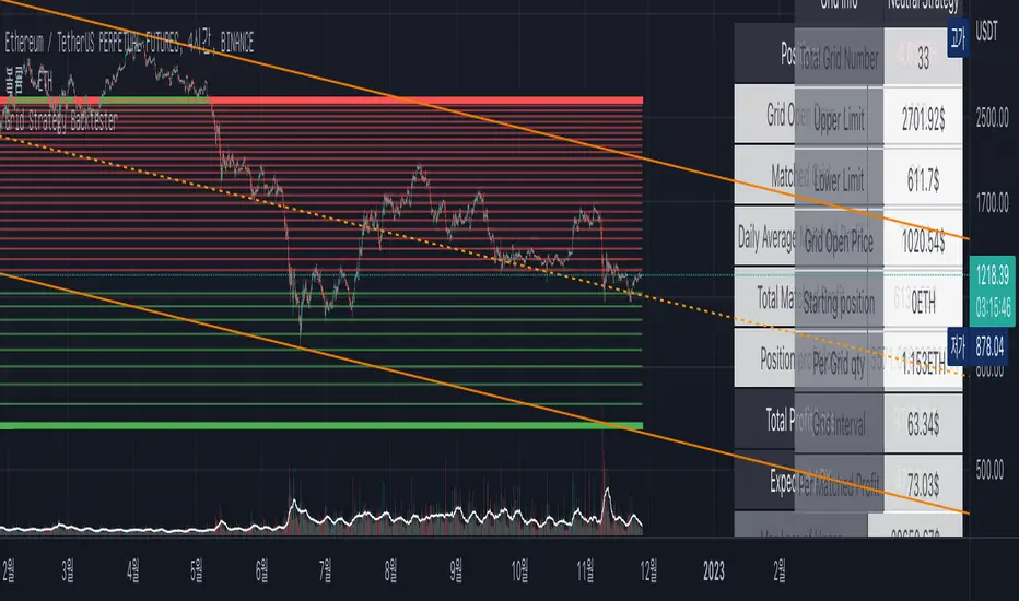
Grid Strategy Back Tester (Long/Short/Neutral)Preface
I'd like to send a thank you to @xxattaxx-DisDev.
The 'Line' Code, which was the most difficult to plan the Grid Indicator, was solved through the 'Grid Bot Simulator' script of @xxattaxx-DisDev.
A brief description of the indicators
These indicators are designed for backtesting of grid trading that can be opened on various exchanges.
Grid trading is a method of selling at particular intervals as prices rise and fall for gird interval price range.
This indicator is actually designed to see what the Long / Short / Neutral grid has achieved and how much it has achieved over a given period of time.
How to use
1. Lower Limit and Upper Limit are required when putting indicators on the chart.
After that, choose the 'Time' when to open the grid.
Also, select Long / Short / Neutral direction if necessary.
2. Statistics Table
Matched Grid shows how many grid pairs were engaged during the backtesting period.
The Daily Average Matching Profit is calculated based on the number of these closed grids.
Total Matching Profit is calculated as Matching Grid * Per Matching Profit.
Position Profit/Loss shows the benefits and losses from your current position.
Total Profit/Loss is sum of Total Matching Profit and Position Profit/Loss.
The Expanded APY shows the benefits of running the strategy on these terms for a year.
Max Loss of Upper is the maximum loss assumed to be directly at the top of the grid range.
BEP days (Upper) show how many days of maintenance relative to Average Matching Profit can result in greater profit than maximum loss if the grid continues to move within range.
(In the case of Long Strategy, it appears to be 'Min Profit', which shows minimal benefit if it reaches the top.)
Max Loss of Lower and BEP days (Lower) shows the opposite.
(In the case of Short Strategy, it is also referred to as 'Min Profit', which shows minimal benefit if it reaches the bottom.)
3. Grid Info
Total Grid Number, Upper Limit, and Lower Limit show the values you set in INPUT.
Grid Open Price shows the price for the period you decide to open.
Starting Position shows the number of positions that were initially held in the case of a Long / Short Strategy.
(0 for Neutral Strategy)
Per Grid qty shows how many positions are allocated to one grid
Grid Interval shows the spacing of each grid.
Per Matched Profit shows how much profit is generated when a single grid is matched.
Caution
Backtesting results for these indicators may vary depending on the time frame.
Therefore, I recommend that you use it only to compare Profit/Loss over time.
*In addition, there is a problem that all lines in the grid are not implemented, but it is independent of the backtest results.
--------------------------------------
서문
지표를 기획함에 있어서 가장 어려웠던 line 코드를 @xxattaxx-DisDev의 'Grid Bot Simulator' 스크립트를 통해 해결할 수 있었습니다.
이에 감사의 말씀을 드립니다.
해당 지표에 대한 간단한 설명
해당 지표는 다양한 거래소에서 오픈할 수 있는 그리드 매매에 대한 백테스팅을 위해 만들어졌습니다.
그리드매매는, 특정 가격 구간에 대해 가격이 오르고 내림에 따라 일정 간격에 맞춰 매매를 하는 방식입니다.
이 지표는 실질적으로 롱/숏/중립 그리드가 어떠한 성과를, 특정 기간동안 얼마나 냈는지를 확인하고자 만들어졌습니다.
사용방법
1. 인풋
지표를 차트위에 넣을 때, Lower Limit과 Upper Limit이 필요합니다.
그 후 그리드를 언제부터 오픈할 것인지를 선택하세요.
또, 필요하다면 Long / Short / Neutral의 방향을 선택하세요.
2. 그리드 통계
Matched Grid는, 백테스팅 기간동안 체결된 그리드 쌍이 몇개인지를 보여줍니다.
이 체결된 그리드의 갯수를 바탕으로 Daily Average Matched Profit이 계산됩니다.
Total Matched Profit은, Matched Grid * Per Matched Profit으로 계산됩니다.
Position Profit/Loss는, 현재 갖고 있는 포지션으로 인한 이익과 손실을 보여줍니다.
Total Matched Profit과 Position Profit/Loss를 합친 금액이 Total Profit/Loss가 됩니다.
Expcted APY는, 이러한 조건으로 전략을 1년동안 운영했을 때의 이익을 보여줍니다.
Max Loss of Upper는, 그리드 범위의 최상단에 바로 도달했을 경우를 가정한 최대 손실입니다.
BEP days(Upper)는, 그리드가 범위 내에서 계속 움직일 경우, Average Matched Profit을 기준으로 며칠동안 유지되어야 최대손실보다 더 큰 이익이 발생할 수 있는지를 보여줍니다.
(Long Strategy의 경우, ‘Min Profit’이라고 나타나는데, 최상단에 도달했을 경우 최소한의 이익을 보여줍니다)
Max Loss of Lower는 그 반대의 경우를 보여줍니다.
(Short Strategy의 경우, 역시 ‘Min Profit’이라고 나타나는데, 최하단에 도착했을 경우 최소한의 이익을 보여줍니다)
3. 그리드 정보
그리드 갯수, Upper Limt, Lower Limt은 자신이 설정한 값을 보여줍니다.
Grid Open Price는, 자신이 오픈하기로 정했던 기간의 가격을 보여줍니다.
Starting Position은, 롱/숏 그리드의 경우에 처음에 들고 시작했던 포지션의 갯수를 보여줍니다.
Neutral Strategy의 경우 0입니다.
Per Grid qty는, 하나의 그리드에 얼마만큼의 포지션이 배분되었는지를 보여주며
Grid Interval은 각 그리드의 간격을 보여줍니다.
또, Per Matched Profit은 하나의 그리드가 체결될 때 얼마만큼의 이익이 발생하는 지를 보여줍니다.
이러한 지표에 대한 역테스트 결과는 시간 프레임에 따라 달라질 수 있습니다.
따라서 시간 경과에 따른 손익을 비교할 때만 사용하는 것이 좋습니다.
*추가로, 그리드의 라인이 모두 구현되지 않는 문제가 있지만, 백테스팅 결과와는 무관합니다.
PineHelperLibrary "PineHelper"
This library provides various functions to reduce your time.
recent_opentrade_entry_bar_index()
get a recent opentrade entry bar_index
Returns: (int) bar_index
recent_closedtrade_entry_bar_index()
get a recent closedtrade entry bar_index
Returns: (int) bar_index
recent_closedtrade_exit_bar_index()
get a recent closedtrade exit bar_index
Returns: (int) bar_index
all_opnetrades_roi()
get all aopentrades roi
Returns: (float) roi
bars_since_recent_opentrade_entry()
get bars since recent opentrade entry
Returns: (int) number of bars
bars_since_recent_closedtrade_entry()
get bars since recent closedtrade entry
Returns: (int) number of bars
bars_since_recent_closedtrade_exit()
get bars since recent closedtrade exit
Returns: (int) number of bars
recent_opentrade_entry_id()
get recent opentrade entry ID
Returns: (string) entry ID
recent_closedtrade_entry_id()
get recent closedtrade entry ID
Returns: (string) entry ID
recent_closedtrade_exit_id()
get recent closedtrade exit ID
Returns: (string) exit ID
recent_opentrade_entry_price()
get recent opentrade entry price
Returns: (float) price
recent_closedtrade_entry_price()
get recent closedtrade entry price
Returns: (float) price
recent_closedtrade_exit_price()
get recent closedtrade exit price
Returns: (float) price
recent_opentrade_entry_time()
get recent opentrade entry time
Returns: (int) time
recent_closedtrade_entry_time()
get recent closedtrade entry time
Returns: (int) time
recent_closedtrade_exit_time()
get recent closedtrade exit time
Returns: (int) time
time_since_recent_opentrade_entry()
get time since recent opentrade entry
Returns: (int) time
time_since_recent_closedtrade_entry()
get time since recent closedtrade entry
Returns: (int) time
time_since_recent_closedtrade_exit()
get time since recent closedtrade exit
Returns: (int) time
recent_opentrade_size()
get recent opentrade size
Returns: (float) size
recent_closedtrade_size()
get recent closedtrade size
Returns: (float) size
all_opentrades_size()
get all opentrades size
Returns: (float) size
recent_opentrade_profit()
get recent opentrade profit
Returns: (float) profit
all_opentrades_profit()
get all opentrades profit
Returns: (float) profit
recent_closedtrade_profit()
get recent closedtrade profit
Returns: (float) profit
recent_opentrade_max_runup()
get recent opentrade max runup
Returns: (float) runup
recent_closedtrade_max_runup()
get recent closedtrade max runup
Returns: (float) runup
recent_opentrade_max_drawdown()
get recent opentrade maxdrawdown
Returns: (float) mdd
recent_closedtrade_max_drawdown()
get recent closedtrade maxdrawdown
Returns: (float) mdd
max_open_trades_drawdown()
get max open trades drawdown
Returns: (float) mdd
recent_opentrade_commission()
get recent opentrade commission
Returns: (float) commission
recent_closedtrade_commission()
get recent closedtrade commission
Returns: (float) commission
qty_by_percent_of_equity(percent)
get qty by percent of equtiy
Parameters:
percent : (series float) percent that you want to set
Returns: (float) quantity
qty_by_percent_of_position_size(percent)
get size by percent of position size
Parameters:
percent : (series float) percent that you want to set
Returns: (float) size
is_day_change()
get bool change of day
Returns: (bool) day is change or not
is_in_trade()
get bool using number of bars
Returns: (bool) allowedToTrade
discord_message(name, message)
get json format discord message
Parameters:
name : (string) name of bot
message : (string) message that you want to send
Returns: (string) json format string
telegram_message(chat_id, message)
get json format telegram message
Parameters:
chat_id : (string) chatId of bot
message : (string) message that you want to send
Returns: (string) json format string

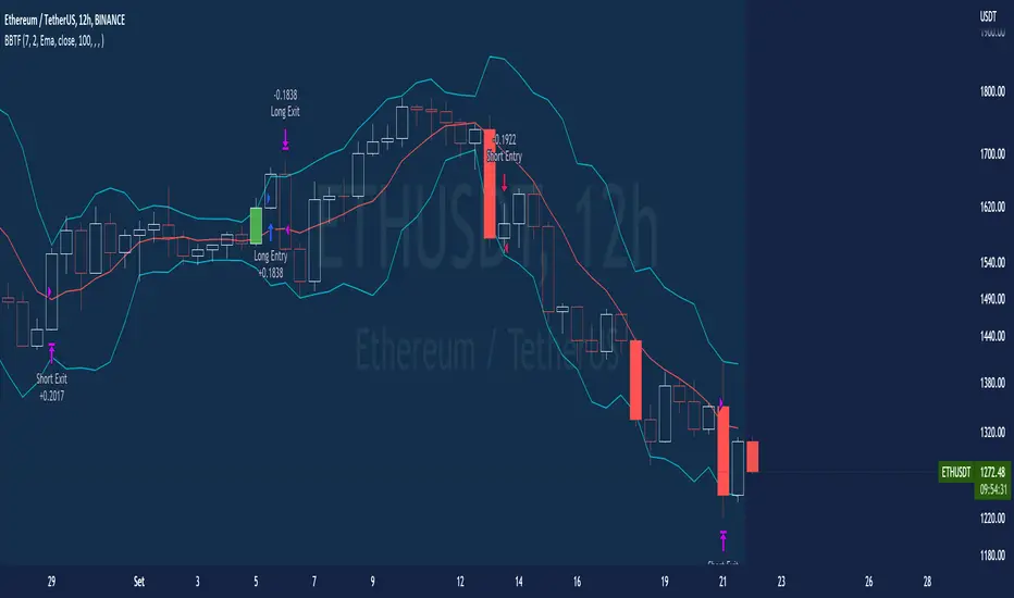
BT-Bollinger Bands - Trend FollowingEsse script foi criado para estudo de Backtest.
O script usa as Bandas de Bollinger para indicar o início de uma tendência, a entrada é configurada quando o preço abre abaixo e fecha acima da banda superior ou para venda quando o preço abre acima e fecha abaixo da banda inferior.
Não há um stop fixo e nem alvo fixo a saída se dá quando o preço toca a média da banda.
Você pode usar uma média móvel como filtro combinado com a estratégia.
O Script também pode ser usado com algum serviço de bot como 3commas.io , basta colocar as mensagens de entrada e saída para o bot.
Autor : Credsonb - Nick: M4TR1X_BR
Neste gráfico estou usando as seguintes configurações:
Bandas Bollinger: 7
Desvio Padrão: 1.5
Time Frame: 12hs
Ticker: ETH
This script was created for Backtest study.
script uses Bollinger Bands to indicate the start of a trend, entry is set when price opens below and closes above the upper band or for short when price opens above and closes below the lower band.
There is no fixed stop and no fixed target, the exit occurs when the price touches the average of the band.
You can use a moving average as a filter combined with the strategy.
The Script can also be used with some bot service like 3commas. io , just put the input and output messages to the bot.
Author : Credsonb - Nick: M4TR1X_BR
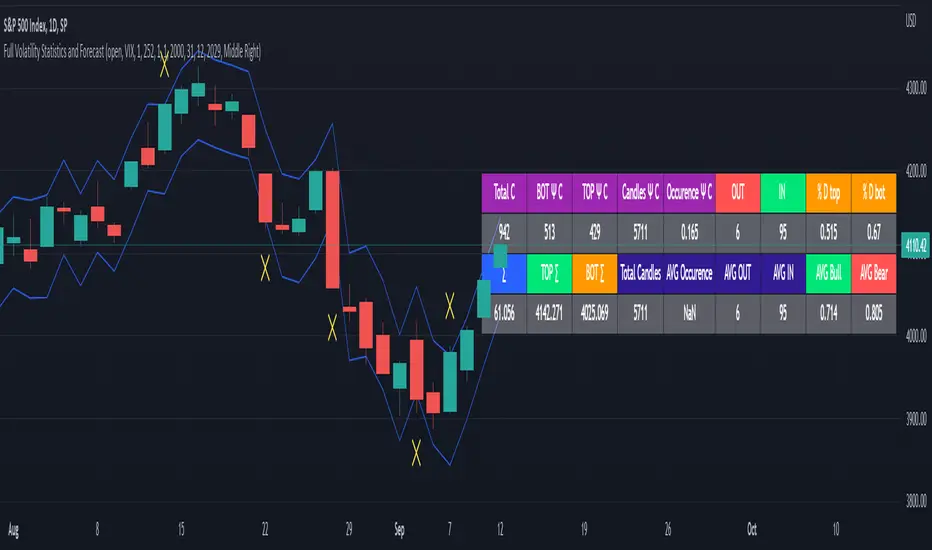
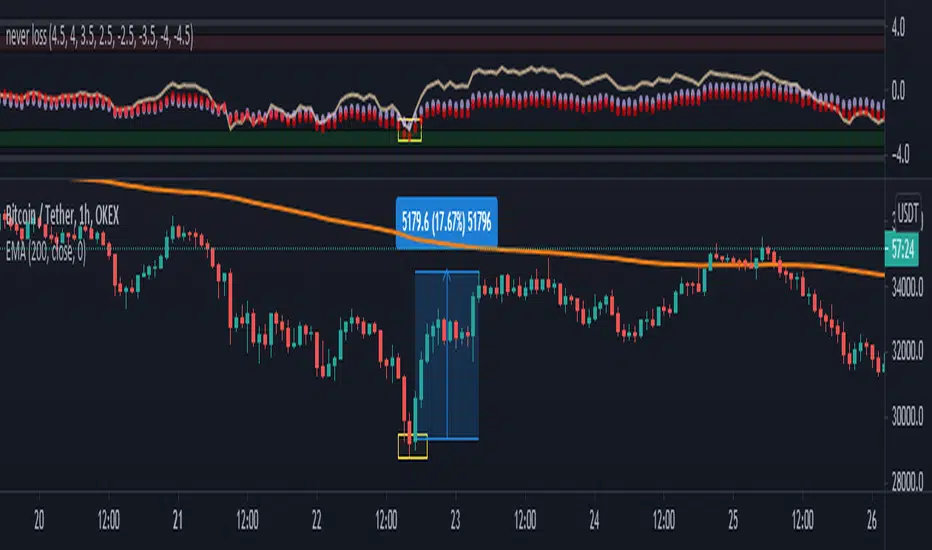
Full Volatility Statistics and Forecast
This is a tool designed to translate the data from the expected volatility of different assets, such as for example VIX, which measures the volatility of SP500 index.
Once get the data from the volatility asset we want to measure(for this test I have used VIX), we are going to translate it the required timeframe expected move by dividing the initial value into :
252 = if we want to use the daily timeframe, since there are ~252 aproximative daily trading days
52 = if we want to use the weekly timeframe, since there 52 trading weeks in a year
12 = if we want to use the monthly timeframe, since there are 12 months in a year
For this example I have used 252 with the daily timeframe.
In this scenario, we can see that we had 5711 total cnadles which we analysed, and in this case, we had 942 crosses, where the daily movement ended up either above or below the channel made from the opening daily candle value + expected movement from the volatility, giving as a total of 16.5% of occurances that volatility was higher than expected, and in 83.5% of the times, we can see that the price stayed within our channel.
At the same time, we can see that we had 6 max losses in a row ( OUT) AND 95 max wins in a row (IN), and at the same time in those moments when the volatility crosses happen we had a 0.51% avg movements when the top crossed happened, and 0.67% avg movements when the bot happened.
Lastly on the second part of the panel, we had E which means the expected movement of today, for example it has 61.056$ , so lets say price opened on 4083, our top is 4083 + 61 and our bot is 4083 - 61 ( giving us the daily channel). At continuation we can see that overall the avg bull candle os 0.714% and avg bear candle was 0.805% .
I hope this tool will help you with your future analysis and trades !
If you have any questions please let me know !
BT-SAR Ema, Squeeze, Volatility
Esse script foi criado para estudo de Backtest.
Ele usa o SAR PARABÓLICO como indicador de sinal de entrada, você também pode combinar 3 indicadores para filtrar as entradas: Média Móvel, Squeeze Momentum e Volatility Oscilator .
Existe duas entradas, quando o SAR Parabólico vira ou pelo Breakout (usando o último preço) do SAR Parabólico antes dele virar.
As Os filtros podem ser usados de forma combinada ou individual.
O Script também pode ser usado com algum serviço de bot como 3commas.io, basta colocar as mensagens de entrada e saída para o bot.
This script was created for Backtest study.
It uses PARABOLIC SAR as input signal indicator, you can also combine 3 indicators to filter inputs: Moving Average, Squeeze Momentum and Volatility Oscillator .
There are two entries, when the Parabolic SAR turns or by Breakout (using the last price) of the Parabolic SAR before it turns.
The Filters can be used in combination or individually.
The Script can also be used with some bot service like 3commas.io, just put the input and output messages to the bot.

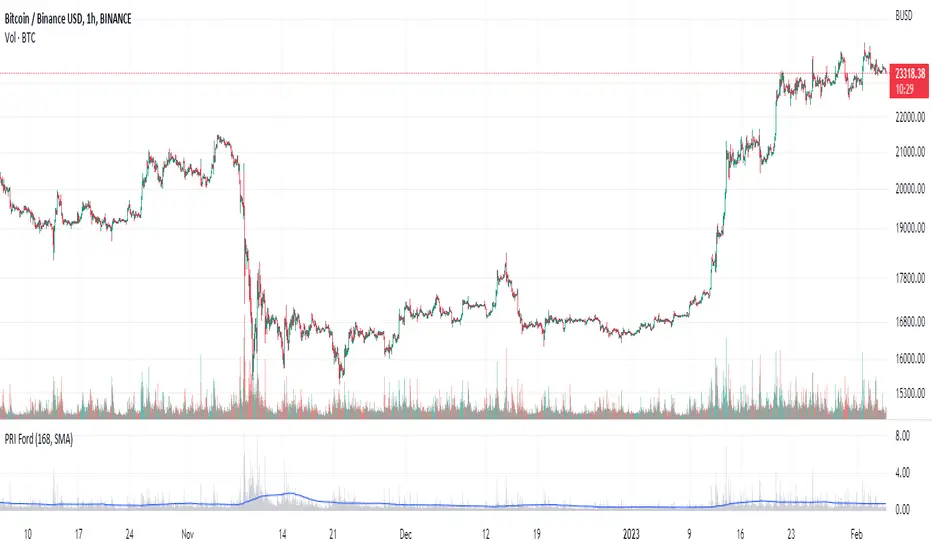
Percentage Range IndicatorThe Percentage Range Indicator is useful for assessing the volatility of pairs for percentage-based grid bots. The higher the percentage range for a given time period, the more trades a grid bot is likely to generate in that period. Conversely, a grid bot can be optimised by using grids that are less than the Percentage Range Indicator value.
I have been using the Percentage Range Indicator based on the one hour time period and 168 periods of smoothing (seven days based on one-hour periods).
Enjoy.
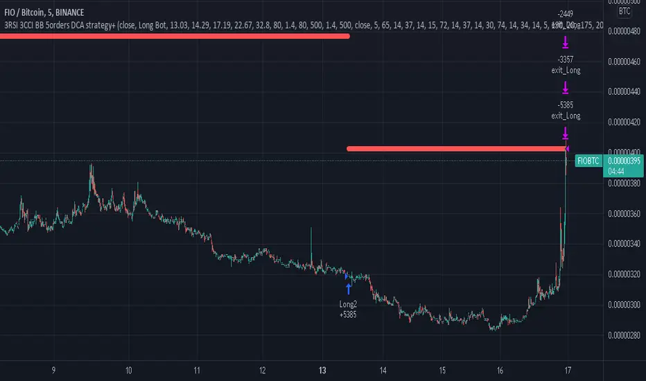
3RSI 3CCI BB 5orders DCA strategy+This strategy is just an attempt to find the indicator values for the trading bot service that I use (link in profile). Due to the use of the “request.security” function in the code, the indicators can be redrawn, but this is not important in history. The strategy used only 5 orders for the "DCA" - bot, located at the same distance in the price overlap range. I only use this strategy when trading in pairs against bitcoin.
Эта стратегия – просто попытка подобрать значения индикаторов для сервиса торговых ботов, который я использую (ссылка в профиле). Из-за использования в коде функции «request.security» возможна перерисовка индикаторов, но на истории это не важно. В стратегии использовано всего 5 ордеров для «DCA» - бота, находящихся на одинаковом расстоянии в диапазоне перекрытия цены. Я использую данную стратегию только при торговле в парах к биткоину.
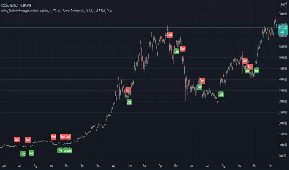
Scalping Trading System ALERT Crypto and StocksThis is the alert version of the strategy with the same name.
Indicators
SImple Moving Average
Exponential Moving Average
Keltner Channels
MACD Histogram
Stochastics
Rules for entry
long= Close of the candle bigger than both moving averages and close of the candle is between the top and bot levels from Keltner . At the same time the macd histogram is negative and stochastic is below 50.
short= Close of the candle smaller than both moving averages and close of the candle is between the top and bot levels from Keltner . At the same time the macd histogram is positive and stochastic is above 50.
Rules for exit
We exit when we meet an opposite reverse order.
This strategy has no risk management inside, so use it with caution !
DiscordWebhookFunctionLibrary "DiscordWebhookFunction"
discordMarkdown(_str, _italic, _bold, _code, _strike, _under) Convert string to markdown formatting User can combine any function at the same time.
Parameters:
_str : String input
_italic : Italic
_bold : Bold
_code : Code markdown
_strike : Strikethrough
_under : Underline
Returns: string Markdown formatted string.
discordWebhookJSON(_username, _avatarImgUrl, _contentText, _bodyTitle, _descText, _bodyUrl, _embedCol, _timestamp, _authorName, _authorUrl, _authorIconUrl, _footerText, _footerIconUrl, _thumbImgUrl, _imageUrl) Convert data to JSON format for Discord Webhook Integration.
Parameters:
_username : Override bot (webhook) username string / name,
_avatarImgUrl : Override bot (webhook) avatar by image URL,
_contentText : Main content page message,
_bodyTitle : Custom Webhook's embed message body title,
_descText : Webhook's embed message body description,
_bodyUrl : Webhook's embed body direct link URL,
_embedCol : Webhook's embed color,
_timestamp : Timestamp,
_authorName : Webhook's embed author name / title,
_authorUrl : Webhook's embed author direct link URL,
_authorIconUrl : Webhook's embed author icon by image URL,
_footerText : Webhook's embed footer text / title,
_footerIconUrl : Webhook's embed footer icon by image URL,
_thumbImgUrl : Webhook's embed thumbnail image URL,
_imageUrl : Webhook's embed body image URL.
Returns: string Single-line JSON format

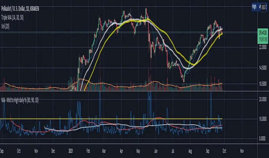
Mid to High daily % - MA & ThresholdPurpose of this script is to provide a metric for comparing crypto volatility in terms of the % gain that can be garnished if you buy the midpoint price of the day and sell the high***. I'm specifically using bots that buy non-stop. This metric makes it easy to compare crypto coins while also providing insight on what a take profit % should be if I want to be sure it closes often instead of getting stuck in a position.
Added a few moving averages of (Mid-range to High Daily %). When these lines starts to trend down, it's time to lower the take profit % or move on to the next coin.
Decided to add a threshold so I could easily mark where I think the (Mid-range to High Daily %) is for most days.
Ex. I can mark 10% threshold and can eyeball roughly ~75% of the days in the past month or so were at or above that level. Then I know I have plenty volatility for a bot taking 5% profit. Also if you have plenty of periodic poke-through that month (let's say once a week) you might argue that you can set it to 7% if you're willing to wait about that long. Either way this metric is conservative because it is only the middle of the range to the high, a less conservative version might provide the % gain if you bought the day low and sold the day high.
***Since this calculation only takes the middle of the range and the high of the day into account, red days are volatile against a buyer but to your advantage if you are a seller. BUT if you have plenty of safety buy orders this volatility in price only means your total purchase volume increases and when/if you reach a take profit level you sell more there.
Would like to upgrade and add a separate MA line for green days and a separate MA line for red days to discern if that particular coin has a bias. Also would like to include some statistics on how many candles are above or below threshold for a certain period instead of eyeballing.
nonoiraq indicator it's very strong i edit this indicator to connect it with my bot to auto trading and he take the info from the volume, so when he is give me a single the bot take just 0.50% to 1% for 3 - 5 trade in day and this perfect, if u use a manual trading this indicator can reach to from 10% to 80% in some point .
the indicator have 3 line
(Red , Purple, Yellow)
1- The yellow line it's high sensitivity this mean it's when rich to the -3 or 3 you can open the order when the bar is close and the signal be sure
and u need to watch the your order because in some case he is reach to 0.30% to 2% and the price reflected to loss and when you wait the price reflected to but my advice you take profit and close the order directly.
2- The purple circles it's medium sensitivity this mean when the purple hit the 2.5 or 3 from down or up in indicator with yellow line you open the order when bar close and the signal is be sure , like example in the photo
3- The red circles it's low sensitivity and this one when reach to 3.0 with any line (yellow or purple) you open directly short or long , like the example in the photo
i am sorry for my english it's not very good
please support me to share other idea or script
Take America Back Version 1.0So basically, the when the price goes down a little, it buys, and when it goes up a little it buys. The only indicators are account balances, and the price, that’s it. Now I wish that Pine Script had a function or variable in which I could recall the balances of specific portions of the portfolio, but it doesn’t. So, I had to improvise. Now for this to work accurately, all of the money needs to be in the “base” side before the bot can begin. Now, the thing about this is that it does not re-invest the amount that is “saved” to all but guarantee the balance will go up. However, as this goes up it will not add up as quickly in order to allow more wiggle room so that the bot does not work itself into a corner. If you want to keep some of your base, enter how much you want to keep it in the initial “saved” setting, as long as you allow at least enough to be equal to the default quantity value. Also, I recommend you setting the pyramiding setting to the result of the base value divided by the default quantity value. The default quantity value is how much you invest, measured in the base currency.
This would have been sooooo much easier if pine script could allow me to recall specific balances, but maybe a future one will.
Finally, THIS is why I made this program, I wanted to create something that would prevent the little ones from being stepped on by the big players who don't always play fair.
Besides, cryptocurrencies were made in response to the 2008 financial meltdown that caused a global recession. This decentralized currency is not just the money of the banks, the corporations, or the governments, but the money of the people. Use this tool to level the massive wealth inequality in my country and take America Back.
I will post more links and updates later once my reputation score goes up. I will discuss more about what influenced me to make this program and as some advise and possible future improvements as well.
