PA Builder [PrimeAutomation]1. PA Builder – Overview
PA Builder is not a fixed strategy; it’s a framework for building strategies. Instead of giving traders one rigid system, it provides a toolbox where entries, exits, filters, risk parameters, and automation rules can all be defined and combined. The core philosophy is confluence: the idea that a trade should only be taken when multiple independent signals agree. The Builder is built around this principle. Every module; trend, reactors, bands, reversals, volume, structure, divergences, externals can be treated as one layer of confidence. The stronger the alignment across layers, the higher the quality of the setup in theory.
In practice, this means PA Builder encourages traders to think in terms of “confluence,” not single indicators. Trend and positioning define whether you should even be looking for longs or shorts. Timing tools such as bands, reversals and candlestick structures determine when inside that broader bias you want to engage. Confirmation tools like volume and flow tell you whether capital is actually supporting the move. Filter systems then ensure that even if everything looks good locally, you still respect higher-timeframe or opposing warnings. The Builder’s philosophy is simple: enter less often, but only when conditions are genuinely in your favour.
2. Core Entry Signal Components
The entry logic in PA Builder is built on a set of signal engines that can be combined in many ways. Trend Signals form a natural foundation. They use low-lag low-pass filters, borrowed from audio signal processing, to extract directional bias from price without the classic delay of classical moving averages. The sensitivity parameter controls how reactive this engine is: lower values favour cleaner trends and fewer whipsaws, while higher values are better suited to short-term intraday trading where speed matters more than smoothness. Many traders start by requiring that Trend Signals show “all bullish” or “all bearish” before allowing any entries in that direction.
Trend signals firing short positions
On top of this directional backbone, the Dynamic Reactor behaves as an adaptive baseline. It accelerates in volatile phases and slows down during consolidation, effectively acting as a moving reference point for both trend and price position. A typical use of this module is to insist that, for long trades, the price sits above a bullish reactor; for shorts, below a bearish one. At the higher-timeframe level, the Quantum Reactor provides a VWAP-style reference that can be anchored to larger candles than the chart you are trading. A common configuration is to trade on a 15-minute chart while requiring that price is above the 4-hour Quantum Reactor for longs or below it for shorts. The “fast” and “slow” options determine how quickly this reference adapts to new information.
Timing is then refined with tools like Quantum Bands, reversals and candle structure analysis. Quantum Bands identify extremes within the current environment. In an uptrend, a tag of the lower band can be treated as a pullback rather than a breakdown; in a downtrend, the upper band acts like a shorting zone. Many traders combine “trend up and above higher-timeframe reactor” with “price temporarily below lower band” to construct a mean-reversion entry inside a larger uptrend. Reversal detection modules examine recent bars to find turning points, with shorter lookbacks capturing fast flips and longer lookbacks tracking deeper structural changes. Candle structure logic goes beyond classical candlestick names and instead focuses on whether price action confirms follow-through or reversion behaviour, with options like “2X” modes that wait for two successive confirmations before acting.
Before and after filtering using reactor applied.
Additional confirmation layers come from Volume Matrix, Money Flow, OSC True7 and divergence detection. Volume and flow tools answer whether actual capital is participating in the move or whether price is drifting on thin activity. OSC True7 categorises the state of the trend into intuitive buckets, strong, healthy, neutral, or exhausted, making it easier to avoid chasing extremes. Divergences between price and momentum can be used either as entry triggers in contrarian systems or as hard filters that block trades when warning signs are present. Finally, two external indicator inputs make it possible to integrate RSI, MACD, custom indicators or even other strategies into the Builder, either as simple thresholds or as comparative logic between two external sources (for example, requiring a fast EMA to be above a slow EMA before allowing longs).
3. Exit System & Trade Management
The exit systems in PA Builder are designed to be as vital as the entry logic. It assumes exits are not an afterthought, but half of the edge. Instead of forcing a single take profit point, the system uses a three-tier structure where you can assign different portions of the position to different targets. A common pattern is to scale out a small portion early (for example at one ATR), another portion at an intermediate level, and keep the largest slice for a deeper move. This creates a natural balance: you book something early to reduce emotional stress, while leaving room to participate in the full potential of a trend.
Targets can be defined using ATR multiples or risk-to-reward ratios that are directly tied to the initial stop distance. Using ATR keeps exits proportional to current volatility. A two ATR target in a quiet environment is very different in absolute price distance from the same multiple in a high-volatility environment, yet conceptually it represents the same “size” move. Risk-to-reward exits build on this by ensuring that if you risk one unit (1R), the reward targets are set at predefined multiples of that risk. This enforces positive expectancy at the structural level: the strategy cannot generate entries with inherently negative payoffs.
Once price begins to move in your favour, trailing logic takes over if you choose to enable it. Trailing can begin immediately from entry or only after a target has been hit. Many users prefer to let TP1 and TP2 behave as fixed profit points and then apply a trailing stop or trailing take profit to the final remainder. That way, routine winners are banked mechanically, while occasional explosive moves can be ridden for as long as the market allows. The breakeven module supports this behaviour by automatically moving stops to entry (or slightly through entry into profit) after a specified condition such as TP1 being hit. This transforms the risk profile mid trade: once breakeven has been secured, remaining size can be managed with much less psychological pressure.
The system also recognises the cost of time. Kill Switch functionality exits trades that have been open too long under mediocre conditions, typically when they are in modest profit but not progressing. This protects you from capital being tied up while better opportunities appear elsewhere. Underlying all of this are several trailing stop mechanisms: percentage-based, tick-based for very short-term strategies, TP linked trailing that activates only once a certain profit threshold has been achieved, and ATR based trailing that automatically scales the trail distance with volatility. Each method serves a slightly different profile of strategy, but all share the same aim: preserve gains and limit downside in a structured way rather than rely on discretionary judgement after the fact.
4. Filters and Risk Management
The filter systems in PA Builder formalise the idea that good trading is often about knowing when not to act. “Do Not Trade” conditions can be configured so that even a perfectly aligned bullish entry stack is overridden if certain bearish evidence is present. These can include higher timeframe reversal structures, powerful opposing divergences, or conflicting signals in key modules. By assigning conditions specifically to “Do Not Long” and “Do Not Short” rather than only to entries, you create asymmetry: buying requires bullish evidence and an absence of strong bearish warnings; selling requires the mirror.
Volatility filters extend this logic to the regime level. Some strategies are inherently suited to low volatility, range bound environments where fading extremes is profitable; others require expansion and energy to function properly. By binding trading permission to volatility ranges, you ensure that a mean-reversion system does not blindly attempt to fade a breakout, and that a momentum system does not spin its wheels in a dead, sideways market. You can even reference volatility from a higher timeframe than the one you trade, so that a five-minute strategy is still aware of the broader one-hour volatility regime it sits inside.
Applied DO NOT TRADE - removes poor signal
Risk management and position sizing are configured so each trade is expressed in units of risk rather than arbitrary size. Leverage, in this framework, is simply a scaling factor for capital efficiency; the actual risk per trade is still controlled by the distance between entry and stop and the percentage of equity you choose to expose. Reinvestment options then decide what proportion of accumulated profit is fed back into position sizing. A more aggressive reinvestment setting accelerates compounding but increases the amplitude of drawdowns; a more conservative one smooths the equity curve at the cost of slower growth. The Base Trade Value parameter ties all of this together by deciding how much nominal capital or how many contracts are committed per trade in light of your maximum allowed simultaneous positions and your intended use of leverage.
External exit conditions provide further flexibility. For example, you might design a system whose entries rely purely on PA Builder’s internal modules, but whose exits use RSI readings, moving average crosses, or a proprietary external indicator. The separation of entry and exit logic allows you to bolt on different behaviours at the tail end of trades while keeping your core signal engine intact. In all cases, the objective is the same: express risk in a controlled, repeatable way that can survive long stretches of unfavourable market conditions.
5. PDT, Cooldowns and Visual Modes
For traders subject to Pattern Day Trading rules, PA Builder includes a day-trade tracking system that counts business days correctly and respects the three-trades-in-five-days limit. This goes beyond simple compliance; it forces discipline. When intraday trading is heavily constrained, you are naturally pushed toward swing-oriented strategies with fewer, more selective entries. The tool visually marks your PDT status so you never inadvertently cross the line and trigger a lockout.
Cooldown systems address another reality: psychological vulnerability after streaks. Following several consecutive wins, many traders unconsciously loosen their standards, take marginal signals, oversize positions, or overtrade. A win-streak cooldown deliberately pauses trading after a configured number of wins, giving you time to reset. The same applies to losing streaks. After a run of losses, the strongest temptation is often to “make it back now,” which is exactly when discipline is weakest. A loss-streak cooldown enforces a break in activity during this high-risk emotional state, helping to prevent cascading damage driven by revenge trading.
Visualisation comes in two main modes. Classic mode emphasises precision: it draws explicit entry lines, stop levels, target levels and fill zones, making it easy to audit risk/reward on each trade, verify that the exit logic behaves as intended, and review historical trades in detail. Modern mode emphasises market feel: instead of focusing on exact levels, it colours candles and backgrounds to reflect momentum, profit state and dynamics.
This helps you see at a glance whether a strategy is operating in a smooth trending environment or a choppy, fragmented one, and whether current trades are broadly working or struggling. Many users develop and debug in Classic mode and then monitor live performance in Modern mode, so both representations become part of the workflow.
6. Strategy Design Workflow, Examples and Cautions
Designing with PA Builder is inherently iterative. You begin with a simple theory and a minimal configuration, perhaps just a trend filter and a basic stop/target structure, and run a backtest. You then examine where the system fails. If you see many losses occurring in counter-trend conditions, you add an additional directional filter or restrict entries with a higher-timeframe reactor condition. If you observe many small whipsaw losses, you might require candle structure confirmation or volume confirmation before allowing an entry. Each change is made one at a time and evaluated. This process gradually builds a layered system where every component has a clear purpose: some reduce drawdown, some increase win rate, some cut out only the worst trades, and others help capture more of the best ones.
A conservative swing strategy might need an agreement between short-term trend signals, a higher-timeframe Quantum position, and a bullish Dynamic Reactor state, while checking that volume supports the move and that no significant bearish reversals or divergences are present on higher timeframes. It might accept relatively few trades, but each trade would be tightly controlled, scaled out over several ATR-based targets and protected with breakeven and trailing logic. On the opposite end, an aggressive scalping configuration would relax some filters, favour faster sensitivities, use short lookback reversals, and tighten stops and targets dramatically, relying on high frequency and careful volatility filtering to maintain edge.
Throughout all of this, overfitting remains the main danger. The more parameters you tune and the more coincidental rules you add to make the backtest equity curve smoother, the more likely it is that you are capturing noise rather than a real, repeatable edge. Signs of overfitting include heavily optimised numeric values with no intuitive justification, large differences between in-sample and out-of-sample results, or strategies that work spectacularly in very specific regimes and collapse elsewhere. To mitigate this, keep strategies as simple as possible, test across different market regimes (bull, bear, range), and accept that robust systems usually look less “perfect” on the historical chart.
Bridging the gap from backtest to live trading is another critical step. Before risking capital, it is wise to paper trade the configuration for a number of trades to confirm that signal frequency, behaviour and execution align with expectations. When going live, starting with minimal size and gradually scaling up based on real-world performance helps manage both financial and psychological risk. If live results diverge significantly from backtest expectations due to slippage, fees, or changing market conditions, you can adjust, reduce size, or temporarily pause rather than commit fully to a failing configuration.
Ultimately, PA Builder is designed to be a tool for building structured, rules-driven trading systems. It gives you the tools to express your ideas, test them, refine them, and run them under controlled risk. It does not remove uncertainty or guarantee results, but it does provide a clear, transparent way to translate trading concepts into executable, testable logic, and to evolve those systems as markets change and your understanding deepens.
Buscar en scripts para "bear"

Reversal Point Dynamics - Machine Learning⇋ Reversal Point Dynamics - Machine Learning
RPD Machine Learning: Self-Adaptive Multi-Armed Bandit Trading System
RPD Machine Learning is an advanced algorithmic trading system that implements genuine machine learning through contextual multi-armed bandits, reinforcement learning, and online adaptation. Unlike traditional indicators that use fixed rules, RPD learns from every trade outcome , automatically discovers which strategies work in current market conditions, and continuously adapts without manual intervention .
Core Innovation: The system deploys six distinct trading policies (ranging from aggressive trend-following to conservative range-bound strategies) and uses LinUCB contextual bandit algorithms with Random Fourier Features to learn which policy performs best in each market regime. After the initial learning phase (50-100 trades), the system achieves autonomous adaptation , automatically shifting between policies as market conditions evolve.
Target Users: Quantitative traders, algorithmic trading developers, systematic traders, and data-driven investors who want a system that adapts over time . Suitable for stocks, futures, forex, and cryptocurrency on any liquid instrument with >100k daily volume.
The Problem This System Solves
Traditional Technical Analysis Limitations
Most trading systems suffer from three fundamental challenges :
Fixed Parameters: Static settings (like "buy when RSI < 30") work well in backtests but may struggle when markets change character. What worked in low-volatility environments may not work in high-volatility regimes.
Strategy Degradation: Manual optimization (curve-fitting) produces systems that perform well on historical data but may underperform in live trading. The system never adapts to new market conditions.
Cognitive Overload: Running multiple strategies simultaneously forces traders to manually decide which one to trust. This leads to hesitation, late entries, and inconsistent execution.
How RPD Machine Learning Addresses These Challenges
Automated Strategy Selection: Instead of requiring you to choose between trend-following and mean-reversion strategies, RPD runs all six policies simultaneously and uses machine learning to automatically select the best one for current conditions. The decision happens algorithmically, removing human hesitation.
Continuous Learning: After every trade, the system updates its understanding of which policies are working. If the market shifts from trending to ranging, RPD automatically detects this through changing performance patterns and adjusts selection accordingly.
Context-Aware Decisions: Unlike simple voting systems that treat all conditions equally, RPD analyzes market context (ADX regime, entropy levels, volatility state, volume patterns, time of day, historical performance) and learns which combinations of context features correlate with policy success.
Machine Learning Architecture: What Makes This "Real" ML
Component 1: Contextual Multi-Armed Bandits (LinUCB)
What Is a Multi-Armed Bandit Problem?
Imagine facing six slot machines, each with unknown payout rates. The exploration-exploitation dilemma asks: Should you keep pulling the machine that's worked well (exploitation) or try others that might be better (exploration)? RPD solves this for trading policies.
Academic Foundation:
RPD implements Linear Upper Confidence Bound (LinUCB) from the research paper "A Contextual-Bandit Approach to Personalized News Article Recommendation" (Li et al., 2010, WWW Conference). This algorithm is used in content recommendation and ad placement systems.
How It Works:
Each policy (AggressiveTrend, ConservativeRange, VolatilityBreakout, etc.) is treated as an "arm." The system maintains:
Reward History: Tracks wins/losses for each policy
Contextual Features: Current market state (8-10 features including ADX, entropy, volatility, volume)
Uncertainty Estimates: Confidence in each policy's performance
UCB Formula: predicted_reward + α × uncertainty
The system selects the policy with highest UCB score , balancing proven performance (predicted_reward) with potential for discovery (uncertainty bonus). Initially, all policies have high uncertainty, so the system explores broadly. After 50-100 trades, uncertainty decreases, and the system focuses on known-performing policies.
Why This Matters:
Traditional systems pick strategies based on historical backtests or user preference. RPD learns from actual outcomes in your specific market, on your timeframe, with your execution characteristics.
Component 2: Random Fourier Features (RFF)
The Non-Linearity Challenge:
Market relationships are often non-linear. High ADX may indicate favorable conditions when volatility is normal, but unfavorable when volatility spikes. Simple linear models struggle to capture these interactions.
Academic Foundation:
RPD implements Random Fourier Features from "Random Features for Large-Scale Kernel Machines" (Rahimi & Recht, 2007, NIPS). This technique approximates kernel methods (like Support Vector Machines) while maintaining computational efficiency for real-time trading.
How It Works:
The system transforms base features (ADX, entropy, volatility, etc.) into a higher-dimensional space using random projections and cosine transformations:
Input: 8 base features
Projection: Through random Gaussian weights
Transformation: cos(W×features + b)
Output: 16 RFF dimensions
This allows the bandit to learn non-linear relationships between market context and policy success. For example: "AggressiveTrend performs well when ADX >25 AND entropy <0.6 AND hour >9" becomes naturally encoded in the RFF space.
Why This Matters:
Without RFF, the system could only learn "this policy has X% historical performance." With RFF, it learns "this policy performs differently in these specific contexts" - enabling more nuanced selection.
Component 3: Reinforcement Learning Stack
Beyond bandits, RPD implements a complete RL framework :
Q-Learning: Value-based RL that learns state-action values. Maps 54 discrete market states (trend×volatility×RSI×volume combinations) to 5 actions (4 policies + no-trade). Updates via Bellman equation after each trade. Converges toward optimal policy after 100-200 trades.
TD(λ) with Eligibility Traces: Extension of Q-Learning that propagates credit backwards through time . When a trade produces an outcome, TD(λ) updates not just the final state-action but all states visited during the trade, weighted by eligibility decay (λ=0.90). This accelerates learning from multi-bar trades.
Policy Gradient (REINFORCE): Learns a stochastic policy directly from 12 continuous market features without discretization. Uses gradient ascent to increase probability of actions that led to positive outcomes. Includes baseline (average reward) for variance reduction.
Meta-Learning: The system learns how to learn by adapting its own learning rates based on feature stability and correlation with outcomes. If a feature (like volume ratio) consistently correlates with success, its learning rate increases. If unstable, rate decreases.
Why This Matters:
Q-Learning provides fast discrete decisions. Policy Gradient handles continuous features. TD(λ) accelerates learning. Meta-learning optimizes the optimization. Together, they create a robust, multi-approach learning system that adapts more quickly than any single algorithm.
Component 4: Policy Momentum Tracking (v2 Feature)
The Recency Challenge:
Standard bandits treat all historical data equally. If a policy performed well historically but struggles in current conditions due to regime shift, the system may be slow to adapt because historical success outweighs recent underperformance.
RPD's Solution:
Each policy maintains a ring buffer of the last 10 outcomes. The system calculates:
Momentum: recent_win_rate - global_win_rate (range: -1 to +1)
Confidence: consistency of recent results (1 - variance)
Policies with positive momentum (recent outperformance) get an exploration bonus. Policies with negative momentum and high confidence (consistent recent underperformance) receive a selection penalty.
Effect: When markets shift, the system detects the shift more quickly through momentum tracking, enabling faster adaptation than standard bandits.
Signal Generation: The Core Algorithm
Multi-Timeframe Fractal Detection
RPD identifies reversal points using three complementary methods :
1. Quantum State Analysis:
Divides price range into discrete states (default: 6 levels)
Peak signals require price in top states (≥ state 5)
Valley signals require price in bottom states (≤ state 1)
Prevents mid-range signals that may struggle in strong trends
2. Fractal Geometry:
Identifies swing highs/lows using configurable fractal strength
Confirms local extremum with neighboring bars
Validates reversal only if price crosses prior extreme
3. Multi-Timeframe Confirmation:
Analyzes higher timeframe (4× default) for alignment
MTF confirmation adds probability bonus
Designed to reduce false signals while preserving valid setups
Probability Scoring System
Each signal receives a dynamic probability score (40-99%) based on:
Base Components:
Trend Strength: EMA(velocity) / ATR × 30 points
Entropy Quality: (1 - entropy) × 10 points
Starting baseline: 40 points
Enhancement Bonuses:
Divergence Detection: +20 points (price/momentum divergence)
RSI Extremes: +8 points (RSI >65 for peaks, <40 for valleys)
Volume Confirmation: +5 points (volume >1.2× average)
Adaptive Momentum: +10 points (strong directional velocity)
MTF Alignment: +12 points (higher timeframe confirms)
Range Factor: (high-low)/ATR × 3 - 1.5 points (volatility adjustment)
Regime Bonus: +8 points (trending ADX >25 with directional agreement)
Penalties:
High Entropy: -5 points (entropy >0.85, chaotic price action)
Consolidation Regime: -10 points (ADX <20, no directional conviction)
Final Score: Clamped to 40-99% range, classified as ELITE (>85%), STRONG (75-85%), GOOD (65-75%), or FAIR (<65%)
Entropy-Based Quality Filter
What Is Entropy?
Entropy measures randomness in price changes . Low entropy indicates orderly, directional moves. High entropy indicates chaotic, unpredictable conditions.
Calculation:
Count up/down price changes over adaptive period
Calculate probability: p = ups / total_changes
Shannon entropy: -p×log(p) - (1-p)×log(1-p)
Normalized to 0-1 range
Application:
Entropy <0.5: Highly ordered (ELITE signals possible)
Entropy 0.5-0.75: Mixed (GOOD signals)
Entropy >0.85: Chaotic (signals blocked or heavily penalized)
Why This Matters:
Prevents trading during choppy, news-driven conditions where technical patterns may be less reliable. Automatically raises quality bar when market is unpredictable.
Regime Detection & Market Microstructure - ADX-Based Regime Classification
RPD uses Wilder's Average Directional Index to classify markets:
Bull Trend: ADX >25, +DI > -DI (directional conviction bullish)
Bear Trend: ADX >25, +DI < -DI (directional conviction bearish)
Consolidation: ADX <20 (no directional conviction)
Transitional: ADX 20-25 (forming direction, ambiguous)
Filter Logic:
Blocks all signals during Transitional regime (avoids trading during uncertain conditions)
Blocks Consolidation signals unless ADX ≥ Min Trend Strength
Adds probability bonus during strong trends (ADX >30)
Effect: Designed to reduce signal frequency while focusing on higher-quality setups.
Divergence Detection
Bearish Divergence:
Price makes higher high
Velocity (price momentum) makes lower high
Indicates weakening upward pressure → SHORT signal quality boost
Bullish Divergence:
Price makes lower low
Velocity makes higher low
Indicates weakening downward pressure → LONG signal quality boost
Bonus: Adds probability points and additional acceleration factor. Divergence signals have historically shown higher success rates in testing.
Hierarchical Policy System - The Six Trading Policies
1. AggressiveTrend (Policy 0):
Probability Threshold: 60% (trades more frequently)
Entropy Threshold: 0.70 (tolerates moderate chaos)
Stop Multiplier: 2.5× ATR (wider stops for trends)
Target Multiplier: 5.0R (larger targets)
Entry Mode: Pyramid (scales into winners)
Best For: Strong trending markets, breakouts, momentum continuation
2. ConservativeRange (Policy 1):
Probability Threshold: 75% (more selective)
Entropy Threshold: 0.60 (requires order)
Stop Multiplier: 1.8× ATR (tighter stops)
Target Multiplier: 3.0R (modest targets)
Entry Mode: Single (one-shot entries)
Best For: Range-bound markets, low volatility, mean reversion
3. VolatilityBreakout (Policy 2):
Probability Threshold: 65% (moderate)
Entropy Threshold: 0.80 (accepts high entropy)
Stop Multiplier: 3.0× ATR (wider stops)
Target Multiplier: 6.0R (larger targets)
Entry Mode: Tiered (splits entry)
Best For: Compression breakouts, post-consolidation moves, gap opens
4. EntropyScalp (Policy 3):
Probability Threshold: 80% (very selective)
Entropy Threshold: 0.40 (requires extreme order)
Stop Multiplier: 1.5× ATR (tightest stops)
Target Multiplier: 2.5R (quick targets)
Entry Mode: Single
Best For: Low-volatility grinding moves, tight ranges, highly predictable patterns
5. DivergenceHunter (Policy 4):
Probability Threshold: 70% (quality-focused)
Entropy Threshold: 0.65 (balanced)
Stop Multiplier: 2.2× ATR (moderate stops)
Target Multiplier: 4.5R (balanced targets)
Entry Mode: Tiered
Best For: Divergence-confirmed reversals, exhaustion moves, trend climax
6. AdaptiveBlend (Policy 5):
Probability Threshold: 68% (balanced)
Entropy Threshold: 0.75 (balanced)
Stop Multiplier: 2.0× ATR (standard)
Target Multiplier: 4.0R (standard)
Entry Mode: Single
Best For: Mixed conditions, general trading, fallback when no clear regime
Policy Clustering (Advanced/Extreme Modes)
Policies are grouped into three clusters based on regime affinity:
Cluster 1 (Trending): AggressiveTrend, DivergenceHunter
High regime affinity (0.8): Performs well when ADX >25
Moderate vol affinity (0.6): Works in various volatility
Cluster 2 (Ranging): ConservativeRange, AdaptiveBlend
Low regime affinity (0.3): Better suited for ADX <20
Low vol affinity (0.4): Optimized for calm markets
Cluster 3 (Breakout): VolatilityBreakout
Moderate regime affinity (0.6): Works in multiple regimes
High vol affinity (0.9): Requires high volatility for optimal characteristics
Hierarchical Selection Process:
Calculate cluster scores based on current regime and volatility
Select best-matching cluster
Run UCB selection within chosen cluster
Apply momentum boost/penalty
This two-stage process reduces learning time - instead of choosing among 6 policies from scratch, system first narrows to 1-2 policies per cluster, then optimizes within cluster.
Risk Management & Position Sizing
Dynamic Kelly Criterion Sizing (Optional)
Traditional Fixed Sizing Challenge:
Using the same position size for all signal probabilities may be suboptimal. Higher-probability signals could justify larger positions, lower-probability signals smaller positions.
Kelly Formula:
f = (p × b - q) / b
Where:
p = win probability (from signal score)
q = loss probability (1 - p)
b = win/loss ratio (average_win / average_loss)
f = fraction of capital to risk
RPD Implementation:
Uses Fractional Kelly (1/4 Kelly default) for safety. Full Kelly is theoretically optimal but can recommend large position sizes. Fractional Kelly reduces volatility while maintaining adaptive sizing benefits.
Enhancements:
Probability Bonus: Normalize(prob, 65, 95) × 0.5 multiplier
Divergence Bonus: Additional sizing on divergence signals
Regime Bonus: Additional sizing during strong trends (ADX >30)
Momentum Adjustment: Hot policies receive sizing boost, cold policies receive reduction
Safety Rails:
Minimum: 1 contract (floor)
Maximum: User-defined cap (default 10 contracts)
Portfolio Heat: Max total risk across all positions (default 4% equity)
Multi-Mode Stop Loss System
ATR Mode (Default):
Stop = entry ± (ATR × base_mult × policy_mult)
Consistent risk sizing
Ignores market structure
Best for: Futures, forex, algorithmic trading
Structural Mode:
Finds swing low (long) or high (short) over last 20 bars
Identifies fractal pivots within lookback
Places stop below/above structure + buffer (0.1× ATR)
Best for: Stocks, instruments that respect structure
Hybrid Mode (Intelligent):
Attempts structural stop first
Falls back to ATR if:
Structural level is invalid (beyond entry)
Structural stop >2× ATR away (too wide)
Best for: Mixed instruments, adaptability
Dynamic Adjustments:
Breakeven: Move stop to entry + 1 tick after 1.0R profit
Trailing: Trail stop 0.8R behind price after 1.5R profit
Timeout: Force close after 30 bars (optional)
Tiered Entry System
Challenge: Equal sizing on all signals may not optimize capital allocation relative to signal quality.
Solution:
Tier 1 (40% of size): Enters immediately on all signals
Tier 2 (60% of size): Enters only if probability ≥ Tier 2 trigger (default 75%)
Example:
Calculated optimal size: 10 contracts
Signal probability: 72%
Tier 2 trigger: 75%
Result: Enter 4 contracts only (Tier 1)
Same signal at 80% probability
Result: Enter 10 contracts (4 Tier 1 + 6 Tier 2)
Effect: Automatically scales size to signal quality, optimizing capital allocation.
Performance Optimization & Learning Curve
Warmup Phase (First 50 Trades)
Purpose: Ensure all policies get tested before system focuses on preferred strategies.
Modifications During Warmup:
Probability thresholds reduced 20% (65% becomes 52%)
Entropy thresholds increased 20% (more permissive)
Exploration rate stays high (30%)
Confidence width (α) doubled (more exploration)
Why This Matters:
Without warmup, system might commit to early-performing policy without testing alternatives. Warmup forces thorough exploration before focusing on best-performing strategies.
Curriculum Learning
Phase 1 (Trades 1-50): Exploration
Warmup active
All policies tested
High exploration (30%)
Learning fundamental patterns
Phase 2 (Trades 50-100): Refinement
Warmup ended, thresholds normalize
Exploration decaying (30% → 15%)
Policy preferences emerging
Meta-learning optimizing
Phase 3 (Trades 100-200): Specialization
Exploration low (15% → 8%)
Clear policy preferences established
Momentum tracking fully active
System focusing on learned patterns
Phase 4 (Trades 200+): Maturity
Exploration minimal (8% → 5%)
Regime-policy relationships learned
Auto-adaptation to market shifts
Stable performance expected
Convergence Indicators
System is learning well when:
Policy switch rate decreasing over time (initially ~50%, should drop to <20%)
Exploration rate decaying smoothly (30% → 5%)
One or two policies emerge with >50% selection frequency
Performance metrics stabilizing over time
Consistent behavior in similar market conditions
System may need adjustment when:
Policy switch rate >40% after 100 trades (excessive exploration)
Exploration rate not decaying (parameter issue)
All policies showing similar selection (not differentiating)
Performance declining despite relaxed thresholds (underlying signal issue)
Highly erratic behavior after learning phase
Advanced Features
Attention Mechanism (Extreme Mode)
Challenge: Not all features are equally important. Trading hour might matter more than price-volume correlation, but standard approaches treat them equally.
Solution:
Each RFF dimension has an importance weight . After each trade:
Calculate correlation: sign(feature - 0.5) × sign(reward)
Update importance: importance += correlation × 0.01
Clamp to range
Effect: Important features get amplified in RFF transformation, less important features get suppressed. System learns which features correlate with successful outcomes.
Temporal Context (Extreme Mode)
Challenge: Current market state alone may be incomplete. Historical context (was volatility rising or falling?) provides additional information.
Solution:
Includes 3-period historical context with exponential decay (0.85):
Current features (weight 1.0)
1 bar ago (weight 0.85)
2 bars ago (weight 0.72)
Effect: Captures momentum and acceleration of market features. System learns patterns like "rising volatility with falling entropy" that may precede significant moves.
Transfer Learning via Episodic Memory
Short-Term Memory (STM):
Last 20 trades
Fast adaptation to immediate regime
High learning rate
Long-Term Memory (LTM):
Condensed historical patterns
Preserved knowledge from past regimes
Low learning rate
Transfer Mechanism:
When STM fills (20 trades), patterns consolidated into LTM . When similar regime recurs later, LTM provides faster adaptation than starting from scratch.
Practical Implementation Guide - Recommended Settings by Instrument
Futures (ES, NQ, CL):
Adaptive Period: 20-25
ML Mode: Advanced
RFF Dimensions: 16
Policies: 6
Base Risk: 1.5%
Stop Mode: ATR or Hybrid
Timeframe: 5-15 min
Forex Majors (EURUSD, GBPUSD):
Adaptive Period: 25-30
ML Mode: Advanced
RFF Dimensions: 16
Policies: 6
Base Risk: 1.0-1.5%
Stop Mode: ATR
Timeframe: 5-30 min
Cryptocurrency (BTC, ETH):
Adaptive Period: 20-25
ML Mode: Extreme (handles non-stationarity)
RFF Dimensions: 32 (captures complexity)
Policies: 6
Base Risk: 1.0% (volatility consideration)
Stop Mode: Hybrid
Timeframe: 15 min - 4 hr
Stocks (Large Cap):
Adaptive Period: 25-30
ML Mode: Advanced
RFF Dimensions: 16
Policies: 5-6
Base Risk: 1.5-2.0%
Stop Mode: Structural or Hybrid
Timeframe: 15 min - Daily
Scaling Strategy
Phase 1 (Testing - First 50 Trades):
Max Contracts: 1-2
Goal: Validate system on your instrument
Monitor: Performance stabilization, learning progress
Phase 2 (Validation - Trades 50-100):
Max Contracts: 2-3
Goal: Confirm learning convergence
Monitor: Policy stability, exploration decay
Phase 3 (Scaling - Trades 100-200):
Max Contracts: 3-5
Enable: Kelly sizing (1/4 Kelly)
Goal: Optimize capital efficiency
Monitor: Risk-adjusted returns
Phase 4 (Full Deployment - Trades 200+):
Max Contracts: 5-10
Enable: Full momentum tracking
Goal: Sustained consistent performance
Monitor: Ongoing adaptation quality
Limitations & Disclaimers
Statistical Limitations
Learning Sample Size: System requires minimum 50-100 trades for basic convergence, 200+ trades for robust learning. Early performance (first 50 trades) may not reflect mature system behavior.
Non-Stationarity Risk: Markets change over time. A system trained on one market regime may need time to adapt when conditions shift (typically 30-50 trades for adjustment).
Overfitting Possibility: With 16-32 RFF dimensions and 6 policies, system has substantial parameter space. Small sample sizes (<200 trades) increase overfitting risk. Mitigated by regularization (λ) and fractional Kelly sizing.
Technical Limitations
Computational Complexity: Extreme mode with 32 RFF dimensions, 6 policies, and full RL stack requires significant computation. May perform slowly on lower-end systems or with many other indicators loaded.
Pine Script Constraints:
No true matrix inversion (uses diagonal approximation for LinUCB)
No cryptographic RNG (uses market data as entropy)
No proper random number generation for RFF (uses deterministic pseudo-random)
These approximations reduce mathematical precision compared to academic implementations but remain functional for trading applications.
Data Requirements: Needs clean OHLCV data. Missing bars, gaps, or low liquidity (<100k daily volume) can degrade signal quality.
Forward-Looking Bias Disclaimer
Reward Calculation Uses Future Data: The RL system evaluates trades using an 8-bar forward-looking window. This means when a position enters at bar 100, the reward calculation considers price movement through bar 108.
Why This is Disclosed:
Entry signals do NOT look ahead - decisions use only data up to entry bar
Forward data used for learning only, not signal generation
In live trading, system learns identically as bars unfold in real-time
Simulates natural learning process (outcomes are only known after trades complete)
Implication: Backtested metrics reflect this 8-bar evaluation window. Live performance may vary if:
- Positions held longer than 8 bars
- Slippage/commissions differ from backtest settings
- Market microstructure changes (wider spreads, different execution quality)
Risk Warnings
No Guarantee of Profit: All trading involves substantial risk of loss. Machine learning systems can fail if market structure fundamentally changes or during unprecedented events.
Maximum Drawdown: With 1.5% base risk and 4% max total risk, expect potential drawdowns. Historical drawdowns do not predict future drawdowns. Extreme market conditions can exceed expectations.
Black Swan Events: System has not been tested under: flash crashes, trading halts, circuit breakers, major geopolitical shocks, or other extreme events. Such events can exceed stop losses and cause significant losses.
Leverage Risk: Futures and forex involve leverage. Adverse moves combined with leverage can result in losses exceeding initial investment. Use appropriate position sizing for your risk tolerance.
System Failures: Code bugs, broker API failures, internet outages, or exchange issues can prevent proper execution. Always monitor automated systems and maintain appropriate safeguards.
Appropriate Use
This System Is:
✅ A machine learning framework for adaptive strategy selection
✅ A signal generation system with probabilistic scoring
✅ A risk management system with dynamic sizing
✅ A learning system designed to adapt over time
This System Is NOT:
❌ A price prediction system (does not forecast exact prices)
❌ A guarantee of profits (can and will experience losses)
❌ A replacement for due diligence (requires monitoring and understanding)
❌ Suitable for complete beginners (requires understanding of ML concepts, risk management, and trading fundamentals)
Recommended Use:
Paper trade for 100 signals before risking capital
Start with minimal position sizing (1-2 contracts) regardless of calculated size
Monitor learning progress via dashboard
Scale gradually over several months only after consistent results
Combine with fundamental analysis and broader market context
Set account-level risk limits (e.g., maximum drawdown threshold)
Never risk more than you can afford to lose
What Makes This System Different
RPD implements academically-derived machine learning algorithms rather than simple mathematical calculations or optimization:
✅ LinUCB Contextual Bandits - Algorithm from WWW 2010 conference (Li et al.)
✅ Random Fourier Features - Kernel approximation from NIPS 2007 (Rahimi & Recht)
✅ Q-Learning, TD(λ), REINFORCE - Standard RL algorithms from Sutton & Barto textbook
✅ Meta-Learning - Learning rate adaptation based on feature correlation
✅ Online Learning - Real-time updates from streaming data
✅ Hierarchical Policies - Two-stage selection with clustering
✅ Momentum Tracking - Recent performance analysis for faster adaptation
✅ Attention Mechanism - Feature importance weighting
✅ Transfer Learning - Episodic memory consolidation
Key Differentiators:
Actually learns from trade outcomes (not just parameter optimization)
Updates model parameters in real-time (true online learning)
Adapts to changing market regimes (not static rules)
Improves over time through reinforcement learning
Implements published ML algorithms with proper citations
Conclusion
RPD Machine Learning represents a different approach from traditional technical analysis to adaptive, self-learning systems . Instead of manually optimizing parameters (which can overfit to historical data), RPD learns behavior patterns from actual trading outcomes in your specific market.
The combination of contextual bandits, reinforcement learning, random fourier features, hierarchical policy selection, and momentum tracking creates a multi-algorithm learning system designed to handle non-stationary markets better than static approaches.
After the initial learning phase (50-100 trades), the system achieves autonomous adaptation - automatically discovering which strategies work in current conditions and shifting allocation without human intervention. This represents an approach where systems adapt over time rather than remaining static.
Use responsibly. Paper trade extensively. Scale gradually. Understand that past performance does not guarantee future results and all trading involves risk of loss.
Taking you to school. — Dskyz, Trade with insight. Trade with anticipation.

coinbot_mr_table이 스크립트는 **"MA 리본(Moving Average Ribbon) 기반 자동매매 전략"**입니다.
이름(coinbot_mr_table)에 모든 기능이 요약되어 있습니다.
coinbot: user_id, exchange, leverage 등 자동매매 봇과 연동하기 위한 웹훅(Webhook) 신호 전송 기능이 포함되어 있습니다.
mr (MA Ribbon): 18개(5~90)의 이동평균선(EMA 또는 SMA)이 100 이평선을 기준으로 정배열/역배열되는지를 색상(LIME/RUBI)으로 구분하여 추세를 판단합니다.
table: 전략의 백테스팅 성과(총 승률, 일일 수익률 등)를 차트 위에 '누적 통계'와 '일일 통계' 테이블로 시각화해 줍니다.
이 스크립트의 매매 로직과 자동매매 신호에 대한 자세한 설명을 한글과 영어로 각각 제공해 드립니다.
🇰🇷 한글 (Korean)
이 스크립트는 **"MA 리본(Moving Average Ribbon)"**을 핵심 엔진으로 사용하는 완전 자동매매(Autotrade) 전략 신호 생성기입니다.
이 지표의 목적은 차트에서 추세를 시각적으로 보여주는 것을 넘어, 구체적인 매매 신호(진입, 분할 익절, 손절)가 발생할 때마다 JSON 형식의 명령어를 자동매매 봇으로 전송하는 것입니다.
1. 📈 매매 전략: MA 리본 추세 추종
이 전략은 18개의 단기/중기 이동평균선(5~90)과 1개의 장기 이동평균선(100)을 사용하여 추세를 정의합니다.
100 이평선: 장기 추세를 가르는 기준선(강/약을 나누는 분수령)입니다.
18개 리본: 이 리본들이 100 이평선 위에서 모두 상승(LIME 색상)하면 '강세 추세', 아래에서 모두 하락(RUBI 색상)하면 '약세 추세'로 판단합니다.
2. 🚦 진입 및 청산 신호
이 전략은 '전환(Reversing)' 전략입니다. 즉, 롱 신호가 발생하면 숏 포지션을 종료하고 롱으로 진입하며, 그 반대도 마찬가지입니다. (항상 롱 또는 숏 포지션을 유지합니다.)
진입 신호 (Long):
추세 확정: 모든 리본이 100 이평선 위에서 '강세(LIME)'로 통일될 때.
재진입 (불타기): 강세 추세 중, 리본이 일시적으로 조정(GREEN)을 보이다가 다시 '강세(LIME)'로 복귀할 때.
진입 신호 (Short):
추세 확정: 모든 리본이 100 이평선 아래에서 '약세(RUBI)'로 통일될 때.
재진입 (물타기): 약세 추세 중, 리본이 일시적으로 반등(MAROON)하다가 다시 '약세(RUBI)'로 복귀할 때.
청산 신호 (자동매매):
진입 (ENTRY): 롱/숏 신호 발생 시, 설정한 user_id, exchange, leverage 등을 포함한 JSON 메시지를 전송합니다.
익절 (TAKE_PROFIT): 롱/숏 포지션이 사용자가 설정한 TP1, TP2, TP3 목표가에 도달하면, 설정된 물량(qty_percent)만큼 분할 익절하라는 JSON 메시지를 전송합니다.
손절 (CLOSE): 포지션이 설정한 sl_percent에 도달하면, 포지션을 즉시 종료하라는 JSON 메시지를 전송합니다.
3. 📊 핵심 기능: 통계 테이블
이 스크립트는 백테스팅 성과를 두 개의 테이블로 요약하여 차트에 실시간으로 표시합니다.
누적 통계 (Total Stats): 전체 기간의 총 진입 횟수, 승/패, 승률(Winrate), 총수익률(Total Profit) 등을 보여줍니다.
일일 통계 (Daily Stats): '오늘' 하루 동안 발생한 매매의 성과(승/패, 승률, 수익률)만 따로 집계하여 보여줍니다.
🇺🇸 영어 (English)
This script is an automated trading (Autotrade) strategy signal generator based on a "Moving Average (MA) Ribbon."
Its purpose extends beyond visual trend analysis; it is designed to generate specific JSON-formatted commands and send them to an automated trading bot whenever a trade signal (entry, take-profit, stop-loss) occurs.
1. 📈 Trading Strategy: MA Ribbon Trend Following
This strategy uses 18 short-to-mid-term Moving Averages (5 to 90) and one long-term Moving Average (100) to define the trend.
100-MA: This acts as the baseline filter, dividing the market into a long-term bull or bear state.
18-MA Ribbon: When all 18 ribbons are above the 100-MA and rising (LIME color), it defines a 'Strong Bull Trend'. When all are below the 100-MA and falling (RUBI color), it defines a 'Strong Bear Trend'.
2. 🚦 Entry and Exit Signals
This is a 'Reversing' strategy. This means when a long signal occurs, it closes any existing short position and enters long, and vice-versa. It is designed to hold a position (either long or short) at all times.
Long Entry Signals:
Trend Confirmation: When all ribbons unify into a 'Strong Bull' (LIME) state above the 100-MA.
Re-entry (Buy the Dip): During a bull trend, if the ribbon shows a temporary pullback (GREEN) and then flips back to 'Strong Bull' (LIME).
Short Entry Signals:
Trend Confirmation: When all ribbons unify into a 'Strong Bear' (RUBI) state below the 100-MA.
Re-entry (Sell the Rally): During a bear trend, if the ribbon shows a temporary rally (MAROON) and then flips back to 'Strong Bear' (RUBI).
Exit Signals (For Automation):
ENTRY: When a long/short signal occurs, it sends a JSON message with the user's user_id, exchange, leverage, etc.
TAKE_PROFIT: When a position reaches the user-defined TP1, TP2, or TP3 price targets, it sends a JSON message to take profit on the specified quantity (qty_percent) for that portion.
CLOSE (Stop-Loss): When a position hits the sl_percent threshold, it sends a JSON message to immediately close the entire position.
3. 📊 Key Feature: Statistics Tables
The script provides two real-time summary tables on the chart to visualize backtesting performance.
Cumulative Stats: Shows lifetime performance, including total trades, wins, losses, win rate, and total profit.
Daily Stats: Isolates and displays the performance metrics (wins, losses, win rate, profit) for "Today's" trading activity only.

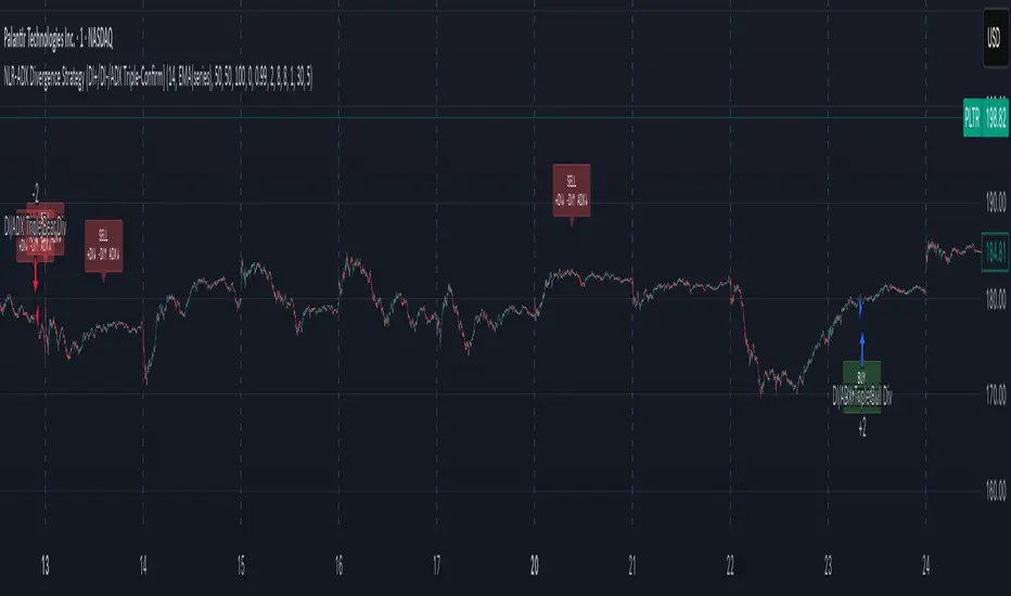
NLR-ADX Divergence Strategy Triple-ConfirmedHow it works
Builds a cleaner DMI/ADX
Recomputes classic +DI, −DI, ADX over a user-set length.
Then “non-linear regresses” each series toward a mean (your choice: dynamic EMA of the series or a fixed Static Mid like 50).
The further a value is from the mean, the stronger the pull (controlled by alphaMin/alphaMax and the γ exponent), giving smoother, more stable DI/ADX lines with less whipsaw.
Optional EMA smoothing on top of that.
Lock in values at confirmed pivots
Uses price pivots (left/right bars) to confirm swing lows and highs.
When a pivot confirms, the script captures (“freezes”) the current +DI, −DI, and ADX values at that bar and stores them. This avoids later drift from smoothing/EMAs.
Check for triple divergence
For a bullish setup (potential long):
Price makes a Lower Low vs. a prior pivot low,
+DI is higher than before (bulls quietly stronger),
−DI is lower (bears weakening),
ADX is lower (trend fatigue).
For a bearish setup (potential short)
Price makes a Higher High,
+DI is lower, −DI is higher,
ADX is lower.
Adds a “no-intersection” sanity check: between the two pivots, the live series shouldn’t snake across the straight line connecting endpoints. This filters messy, low-quality structures.
Trade logic
On a valid triple-confirm, places a strategy.entry (Long for bullish, Short for bearish) and optionally labels the bar (BUY or SELL with +DI/−DI/ADX arrows).
Simple flip behavior: if you’re long and a new short signal prints (or vice versa), it closes the open side and flips.
Key inputs you can tweak
Custom DMI Settings
DMI Length — base length for DI/ADX.
Non-Linear Regression Model
Mean Reference — EMA(series) (dynamic) or Static mid (e.g., 50).
Dynamic Mean Length & Deviation Scale Length — govern the mean and scale used for regression.
Min/Max Regression & Non-Linearity Exponent (γ) — how strongly values are pulled toward the mean (stronger when far away).
Divergence Engine
Pivot Left/Right Bars — how strict the swing confirmation is (larger = more confirmation, more delay).
Min Bars Between Pivots — avoids comparing “near-duplicate” swings.
Max Historical Pivots to Store — memory cap.
CBC Flip StrategyThe CBC Flip Strategy is a momentum-based trading system that identifies shifts in market control by monitoring price closes relative to previous bars' highs and lows: it flips to bullish mode when the close exceeds the prior high (indicating bulls in control) and enters a long position, or to bearish mode when the close falls below the prior low (indicating bears in control) and enters a short position, all while incorporating optional confluences like higher timeframe CBC alignment, RSI thresholds (above 50 + offset for longs, below 50 - offset for shorts), and EMA positioning (above for longs, below for shorts) to filter entries; trades are restricted to a user-defined session window and direction preferences, with exits handled via tick-based TP/SL, reversal on chart or higher timeframe CBC flips, and an optional flatten at a specified time to close all positions.
Number of Contracts: Adjust the quantity of contracts per trade (default: 1).
SL and TP Ticks: Set stop-loss (default: 12 ticks) and take-profit (default: 24 ticks) distances from entry.
Exit Strategy: Choose from TP/SL in ticks, exit on chart CBC flip (reverses on opposite signal), or exit on higher timeframe CBC flip.
Flatten All: Enable/disable flattening all positions at a customizable time (default: 16:00, with adjustable hour/minute).
Trading Session: Define the time window for allowing entries (default: 0800-1700).
Trade Direction: Select "Both" (longs and shorts), "Only Long", "Only Short", or "Towards Daily Open" (longs if below daily open, shorts if above).
Higher Timeframe CBC Confluence: Toggle use of HTF CBC alignment (default: enabled, with customizable HTF like "240").
RSI Confluence: Toggle RSI filter (default: enabled, with adjustable length=14, offset=20 for thresholds).
EMA Confluence: Toggle EMA filter (default: enabled, with adjustable length=200 for position relative to price).

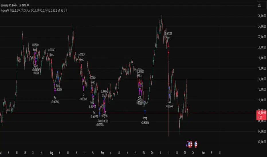
Hyper SAR Reactor Trend StrategyHyperSAR Reactor Adaptive PSAR Strategy
Summary
Adaptive Parabolic SAR strategy for liquid stocks, ETFs, futures, and crypto across intraday to daily timeframes. It acts only when an adaptive trail flips and confirmation gates agree. Originality comes from a logistic boost of the SAR acceleration using drift versus ATR, plus ATR hysteresis, inertia on the trail, and a bear-only gate for shorts. Add to a clean chart and run on bar close for conservative alerts.
Scope and intent
• Markets: large cap equities and ETFs, index futures, major FX, liquid crypto
• Timeframes: one minute to daily
• Default demo: BTC on 60 minute
• Purpose: faster yet calmer PSAR that resists chop and improves short discipline
• Limits: this is a strategy that places simulated orders on standard candles
Originality and usefulness
• Novel fusion: PSAR AF is boosted by a logistic function of normalized drift, trail is monotone with inertia, entries use ATR buffers and optional cooldown, shorts are allowed only in a bear bias
• Addresses false flips in low volatility and weak downtrends
• All controls are exposed in Inputs for testability
• Yardstick: ATR normalizes drift so settings port across symbols
• Open source. No links. No solicitation
Method overview
Components
• Adaptive AF: base step plus boost factor times logistic strength
• Trail inertia: one sided blend that keeps the SAR monotone
• Flip hysteresis: price must clear SAR by a buffer times ATR
• Volatility gate: ATR over its mean must exceed a ratio
• Bear bias for shorts: price below EMA of length 91 with negative slope window 54
• Cooldown bars optional after any entry
• Visual SAR smoothing is cosmetic and does not drive orders
Fusion rule
Entry requires the internal flip plus all enabled gates. No weighted scores.
Signal rule
• Long when trend flips up and close is above SAR plus buffer times ATR and gates pass
• Short when trend flips down and close is below SAR minus buffer times ATR and gates pass
• Exit uses SAR as stop and optional ATR take profit per side
Inputs with guidance
Reactor Engine
• Start AF 0.02. Lower slows new trends. Higher reacts quicker
• Max AF 1. Typical 0.2 to 1. Caps acceleration
• Base step 0.04. Typical 0.01 to 0.08. Raises speed in trends
• Strength window 18. Typical 10 to 40. Drift estimation window
• ATR length 16. Typical 10 to 30. Volatility unit
• Strength gain 4.5. Typical 2 to 6. Steepness of logistic
• Strength center 0.45. Typical 0.3 to 0.8. Midpoint of logistic
• Boost factor 0.03. Typical 0.01 to 0.08. Adds to step when strength rises
• AF smoothing 0.50. Typical 0.2 to 0.7. Adds inertia to AF growth
• Trail smoothing 0.35. Typical 0.15 to 0.45. Adds inertia to the trail
• Allow Long, Allow Short toggles
Trade Filters
• Flip confirm buffer ATR 0.50. Typical 0.2 to 0.8. Raise to cut flips
• Cooldown bars after entry 0. Typical 0 to 8. Blocks re entry for N bars
• Vol gate length 30 and Vol gate ratio 1. Raise ratio to trade only in active regimes
• Gate shorts by bear regime ON. Bear bias window 54 and Bias MA length 91 tune strictness
Risk
• TP long ATR 1.0. Set to zero to disable
• TP short ATR 0.0. Set to 0.8 to 1.2 for quicker shorts
Usage recipes
Intraday trend focus
Confirm buffer 0.35 to 0.5. Cooldown 2 to 4. Vol gate ratio 1.1. Shorts gated by bear regime.
Intraday mean reversion focus
Confirm buffer 0.6 to 0.8. Cooldown 4 to 6. Lower boost factor. Leave shorts gated.
Swing continuation
Strength window 24 to 34. ATR length 20 to 30. Confirm buffer 0.4 to 0.6. Use daily or four hour charts.
Properties visible in this publication
Initial capital 10000. Base currency USD. Order size Percent of equity 3. Pyramiding 0. Commission 0.05 percent. Slippage 5 ticks. Process orders on close OFF. Bar magnifier OFF. Recalculate after order filled OFF. Calc on every tick OFF. No security calls.
Realism and responsible publication
No performance claims. Past results never guarantee future outcomes. Shapes can move while a bar forms and settle on close. Strategies execute only on standard candles.
Honest limitations and failure modes
High impact events and thin books can void assumptions. Gap heavy symbols may prefer longer ATR. Very quiet regimes can reduce contrast and invite false flips.
Open source reuse and credits
Public domain building blocks used: PSAR concept and ATR. Implementation and fusion are original. No borrowed code from other authors.
Strategy notice
Orders are simulated on standard candles. No lookahead.
Entries and exits
Long: flip up plus ATR buffer and all gates true
Short: flip down plus ATR buffer and gates true with bear bias when enabled
Exit: SAR stop per side, optional ATR take profit, optional cooldown after entry
Tie handling: stop first if both stop and target could fill in one bar
Master Trend Strategy - by jake_thebossMaster Trend Strategy
This strategy combines multiple technical indicators to identify high-probability trend entries across all asset classes.
Core Signal Logic:
Entry triggered when EMA 4 crosses above/below EMA 5
Confirmation required from RSI (>50 for long, <50 for short)
Price must be above/below key moving averages: EMA 21, SMA 50, EMA 55, EMA 89, and EMA 750
Additional confirmation from Stochastic (>52 bullish, <48 bearish) or EMA 89 breakout or VWAP cross
Key Features:
VWAP filter: Only takes bullish signals above VWAP and bearish signals below VWAP
Optional pyramiding: Allows multiple entries in the same direction (up to 200 orders)
Individual stop loss and take profit management for each pyramid level
Time filter: Customizable trading hours with timezone offset
Risk management: Adjustable stop loss (default 0.3%) and take profit (default 0.6%)
Visualization:
Entry, stop loss, and take profit levels drawn as horizontal lines
Customizable signal markers (triangles) for bull/bear entries
Optional EMA overlay display
The strategy is designed for trend-following on lower timeframes, with strict multi-indicator confirmation to filter out false signals.

AlgoWay GRSIM🧭 What this strategy tries to do
This strategy detects when a market move is losing strength and prepares for a potential reversal, but it waits for fresh momentum confirmation before acting.
It combines:
• RSI-based divergence (to spot exhaustion and potential turning points),
• Impulse MACD (to verify that the new direction actually has force behind it).
________________________________________
⚙️ When it takes trades
Long (Buy):
• A bullish RSI divergence appears (a clue that selling pressure is fading);
• Within a short time window, the Impulse MACD turns strongly positive;
• Optionally, the impulse line itself must be rising (if the Impulse Direction Filter is
enabled).
Short (Sell):
• A bearish RSI divergence appears (buying pressure fading);
• Within a short time window, the Impulse MACD turns strongly negative;
• Optionally, the impulse line must be falling (if the Impulse Direction Filter is enabled).
If momentum confirmation happens too late, the divergence “expires” and the signal is ignored.
________________________________________
🧩 How entries work
1. Reversal clue:
The strategy detects disagreement between price and RSI (price makes a new high/low, RSI doesn’t).
That suggests a shift in underlying strength.
2. Momentum confirmation:
Before entering, the Impulse MACD must agree — showing real push in the same direction.
3. Impulse direction filter (optional):
When enabled, the impulse itself must accelerate (rise for longs, fall for shorts), avoiding fake signals where price diverges but momentum is still fading.
4. No stacking:
It opens only one position at a time.
________________________________________
🚪 How exits work
Two main exit styles:
Conservative (default):
Longs close when impulse crosses below its signal line.
Shorts close when impulse crosses above its signal line.
✅ Keeps trades as long as momentum agrees.
Color-change (fast):
Longs close immediately when impulse flips bearish.
Shorts close immediately when impulse flips bullish.
⚡ Faster and more defensive.
Plus:
Stop Loss (%) and Take Profit (%) act as fixed-distance protective exits (set to 0 to disable either one).
________________________________________
📊 What you’ll see on the chart
A thick Impulse MACD line and thin signal line (oscillator view).
Diamonds — detected bullish/bearish divergence points.
Circles — where impulse crosses its signal (momentum change).
A performance panel (top-right) showing Net Profit, Trades, Win Rate, Profit Factor, Pessimistic PF, and Max Drawdown.
________________________________________
🔧 What you can tune
Signal Lifetime (bars): how long a divergence remains valid.
Impulse Direction Filter: ensure the impulse itself is moving in the trade’s direction.
Stop Loss / Take Profit (%): risk and target in percent.
Exit Style: conservative cross or faster color-change.
RSI / MA / Signal Lengths: adjust responsiveness (defaults are balanced).
________________________________________
💪 Strengths
Confirms reversals using momentum direction, not just divergence.
Avoids “early” signals where momentum is still fading.
Works symmetrically for longs and shorts.
Built-in stop/target protection.
Clear, visual confirmation of all logic components.
________________________________________
⚠️ Things to keep in mind
In sideways markets, the impulse can flip often — prefer conservative exits.
Too small SL/TP → constant stop-outs.
Too wide SL/TP → deep drawdowns.
Always test with different timeframes and markets.
________________________________________
💡 Practical tips
Start with default settings.
Enable “Use Impulse Direction Filter” in trending markets, disable it in very choppy ones.
Focus on Profit Factor, Win Rate, and Max Drawdown after several dozen trades.
Keep SL/TP roughly aligned with typical swing size.
“AlgoWay GRSIM” is a reversal-with-confirmation strategy: it spots likely turns, demands real momentum alignment (optionally verified by impulse direction), and manages exits with clear momentum cues plus built-in protective limits.

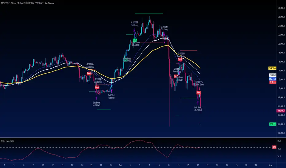
Turtle Strategy - Triple EMA Trend with ADX and ATRDescription
The Triple EMA Trend strategy is a directional momentum system built on the alignment of three exponential moving averages and a strong ADX confirmation filter. It is designed to capture established trends while maintaining disciplined risk management through ATR-based stops and targets.
Core Logic
The system activates only under high-trend conditions, defined by the Average Directional Index (ADX) exceeding a configurable threshold (default: 43).
A bullish setup occurs when the short-term EMA is above the mid-term EMA, which in turn is above the long-term EMA, and price trades above the fastest EMA.
A bearish setup is the mirror condition.
Execution Rules
Entry:
• Long when ADX confirms trend strength and EMA alignment is bullish.
• Short when ADX confirms trend strength and EMA alignment is bearish.
Exit:
• Stop Loss: 1.8 × ATR below (for longs) or above (for shorts) the entry price.
• Take Profit: 3.3 × ATR in the direction of the trade.
Both parameters are configurable.
Additional Features
• Start/end date inputs for controlled backtesting.
• Selective activation of long or short trades.
• Built-in commission and position sizing (percent of equity).
• Full visual representation of EMAs, ADX, stop-loss, and target levels.
This strategy emphasizes clean trend participation, strict entry qualification, and consistent reward-to-risk structure. Ideal for swing or medium-term testing across trending assets.
Larry Williams Oops StrategyThis strategy is a modern take on Larry Williams’ classic Oops setup. It trades intraday while referencing daily bars to detect opening gaps and align entries with the prior day’s direction. Risk is managed with day-based stops, and—unlike the original—all positions are closed at the end of the session (or at the last bar’s close), not at a fixed profit target or the first profitable open.
Entry Rules
Long setup (bullish reversion): Today opens below yesterday’s low (down gap) and yesterday’s candle was bearish. Place a buy stop at yesterday’s low + Filter (ticks).
Short setup (bearish reversion): Today opens above yesterday’s high (up gap) and yesterday’s candle was bullish. Place a sell stop at yesterday’s high − Filter (ticks).
Longs are only taken on down-gap days; shorts only on up-gap days.
Protective Stop
If long, stop loss trails the current day’s low.
If short, stop loss trails the current day’s high.
Exit Logic
Positions are force-closed at the end of the session (in the last bar), ensuring no overnight exposure. There is no take-profit; only stop loss or end-of-day flat.
Notes
This strategy is designed for intraday charts (minutes/seconds) using daily data for gaps and prior-day direction.
Longs/shorts can be enabled or disabled independently.

Batman Strategy v1
1. Overview & Core Concept
The "Batman Strategy V1" is a comprehensive trend-following and pyramid-trading framework designed for multiple asset classes. Its core concept is to identify strong, established trends and systematically enter positions in stages (pyramiding) to maximize gains during sustained market movements.
This strategy is built on a proprietary scoring system that synthesizes multiple market dimensions—including stage analysis, relative strength, and volume dynamics—into clear, actionable signals. It is not a simple indicator mashup; it's a complete system with defined entry, exit, and risk management protocols.
2. Key Features
Proprietary Trend Scoring: The strategy grades market conditions from 'A' (strong bull trend) to 'Z' (strong bear trend) using a unique combination of ADX and RSI calculations, providing a nuanced view of trend maturity and strength.
Advanced Relative Strength Analysis: Automatically compares the asset's performance against a relevant market index (e.g., NIFTY for Indian stocks, NDX for US stocks, or a total crypto market cap for crypto) to ensure it is a market leader.
Heikin-Ashi Based Logic: Utilizes Heikin-Ashi candles for its core calculations to filter out market noise and provide smoother trend signals.
Multi-Tranche Pyramiding: The strategy is designed to enter a position with an initial tranche and add up to four subsequent positions if the trend continues favorably, based on a proprietary breakout logic (`ha_close > breakout`).
Dynamic & Multi-Option Exits: Offers three distinct, user-selectable trailing stop mechanisms for exits: SuperTrend, V-Stop, and Chandelier Exit. This allows traders to tailor the exit logic to their risk tolerance and the asset's volatility. The data source for these exits can also be switched between the standard chart and Heikin-Ashi candles.
Integrated Risk Management: Implements a sophisticated stop-loss system that adjusts based on the number of open trades, aiming to move to break-even after the third tranche and protecting capital.
3. How to Use This Strategy
Configuration: In the script settings, first set your desired backtesting date range. Then, configure the "Entry," "Tranching," and "Exit" parameters to suit your trading style. The most important choice is the "Exit Indicator," as this will define how the strategy closes trades.
Interpretation: When applied to a chart, the strategy will plot trend score labels ('A', 'B', 'C' for bullish; 'X', 'Y', 'Z' for bearish), color the background based on relative strength, and color the bars based on volume strength. Backtesting results, including all pyramided trades, will be visible in the "Strategy Tester" panel.
Alerts: The script includes built-in alert conditions for both bullish and bearish trend scores, which can be used to notify you of potential opportunities.
4. Backtesting & Performance
This is a strategy script, and its performance should be thoroughly evaluated in the Strategy Tester. As per TradingView rules, users should use realistic settings for initial capital, commission, and slippage. The default settings are a template; they should be adjusted to reflect the conditions of the market you are testing. Past performance is not indicative of future results.
5. Disclaimer
This strategy is a tool for market analysis and idea validation. It is not financial advice. All trading involves risk, and you should not risk more than you are prepared to lose. This is a closed-source, protected script; its internal calculations are proprietary.

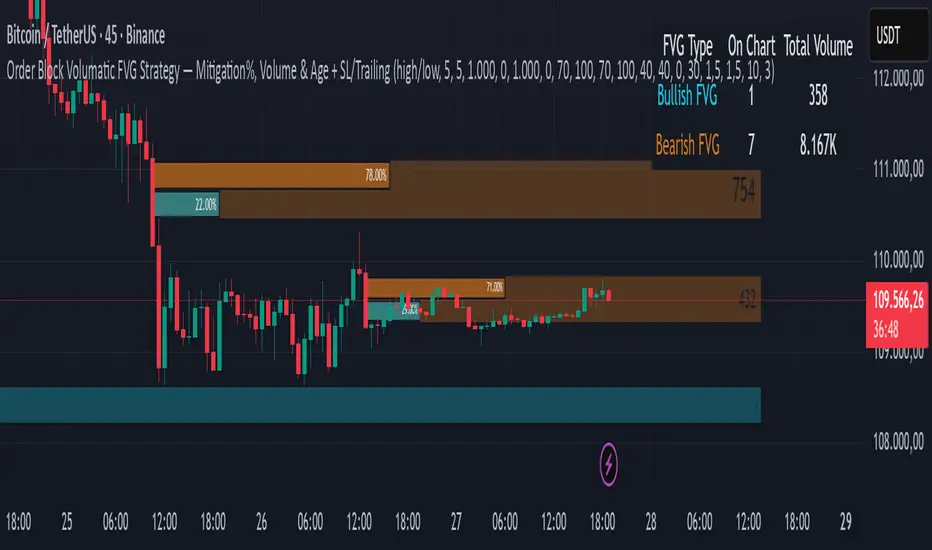
Order Block Volumatic FVG StrategyInspired by: Volumatic Fair Value Gaps —
License: CC BY-NC-SA 4.0 (Creative Commons Attribution–NonCommercial–ShareAlike).
This script is a non-commercial derivative work that credits the original author and keeps the same license.
What this strategy does
This turns BigBeluga’s visual FVG concept into an entry/exit strategy. It scans bullish and bearish FVG boxes, measures how deep price has mitigated into a box (as a percentage), and opens a long/short when your mitigation threshold and filters are satisfied. Risk is managed with a fixed Stop Loss % and a Trailing Stop that activates only after a user-defined profit trigger.
Additions vs. the original indicator
✅ Strategy entries based on % mitigation into FVGs (long/short).
✅ Lower-TF volume split using upticks/downticks; fallback if LTF data is missing (distributes prior bar volume by close’s position in its H–L range) to avoid NaN/0.
✅ Per-FVG total volume filter (min/max) so you can skip weak boxes.
✅ Age filter (min bars since the FVG was created) to avoid fresh/immature boxes.
✅ Bull% / Bear% share filter (the 46%/53% numbers you see inside each FVG).
✅ Optional candle confirmation and cooldown between trades.
✅ Risk management: fixed SL % + Trailing Stop with a profit trigger (doesn’t trail until your trigger is reached).
✅ Pine v6 safety: no unsupported args, no indexof/clamp/when, reverse-index deletes, guards against zero/NaN.
How a trade is decided (logic overview)
Detect FVGs (same rules as the original visual logic).
For each FVG currently intersected by the bar, compute:
Mitigation % (how deep price has entered the box).
Bull%/Bear% split (internal volume share).
Total volume (printed on the box) from LTF aggregation or fallback.
Age (bars) since the box was created.
Apply your filters:
Mitigation ≥ Long/Short threshold.
Volume between your min and max (if enabled).
Age ≥ min bars (if enabled).
Bull% / Bear% within your limits (if enabled).
(Optional) the current candle must be in trade direction (confirm).
If multiple FVGs qualify on the same bar, the strategy uses the most recent one.
Enter long/short (no pyramiding).
Exit with:
Fixed Stop Loss %, and
Trailing Stop that only starts after price reaches your profit trigger %.
Input settings (quick guide)
Mitigation source: close or high/low. Use high/low for intrabar touches; close is stricter.
Mitigation % thresholds: minimal mitigation for Long and Short.
TOTAL Volume filter: skip FVGs with too little/too much total volume (per box).
Bull/Bear share filter: require, e.g., Long only if Bull% ≥ 50; avoid Short when Bull% is high (Short Bull% max).
Age filter (bars): e.g., ≥ 20–30 bars to avoid fresh boxes.
Confirm candle: require candle direction to match the trade.
Cooldown (bars): minimum bars between entries.
Risk:
Stop Loss % (fixed from entry price).
Activate trailing at +% profit (the trigger).
Trailing distance % (the trailing gap once active).
Lower-TF aggregation:
Auto: TF/Divisor → picks 1/3/5m automatically.
Fixed: choose 1/3/5/15m explicitly.
If LTF can’t be fetched, fallback allocates prior bar’s volume by its close position in the bar’s H–L.
Suggested starting presets (you should optimize per market)
Mitigation: 60–80% for both Long/Short.
Bull/Bear share:
Long: Bull% ≥ 50–70, Bear% ≤ 100.
Short: Bull% ≤ 60 (avoid shorting into strong support), Bear% ≥ 0–70 as you prefer.
Age: ≥ 20–30 bars.
Volume: pick a min that filters noise for your symbol/timeframe.
Risk: SL 4–6%, trailing trigger 1–2%, distance 1–2% (crypto example).
Set slippage/fees in Strategy Properties.
Notes, limitations & best practices
Data differences: The LTF split uses request.security_lower_tf. If the exchange/data feed has sparse LTF data, the fallback kicks in (it’s deliberate to avoid NaNs but is a heuristic).
Real-time vs backtest: The current bar can update until close; results on historical bars use closed data. Use “Bar Replay” to understand intrabar effects.
No pyramiding: Only one position at a time. Modify pyramiding in the header if you need scaling.
Assets: For spot/crypto, TradingView “volume” is exchange volume; in some markets it may be tick volume—interpret filters accordingly.
Risk disclosure: Past performance ≠ future results. Use appropriate position sizing and risk controls; this is not financial advice.
Credits
Visual FVG concept and original implementation: BigBeluga.
This derivative strategy adds entry/exit logic, volume/age/share filters, robust LTF handling, and risk management while preserving the original spirit.
License remains CC BY-NC-SA 4.0 (non-commercial, attribution required, share-alike).
Grand Master's Candlestick Dominance (ATR Enhanced)### Grand Master's Candlestick Dominance (ATR Enhanced)
**Overview**
Unleash the ancient wisdom of Japanese candlestick charting with a modern twist! This comprehensive Pine Script v5 strategy and indicator scans for over 75 classic and advanced candlestick patterns (bullish, bearish, and neutral), assigning dynamic strength scores (1-10) to each for precise signal filtering. Enhanced with Average True Range (ATR) for volatility-aware body size validation, it dominates the markets by combining timeless pattern recognition with robust confirmation layers. Whether used as a backtestable strategy or visual indicator, it empowers traders to spot high-probability reversals, continuations, and indecision setups with surgical accuracy.
Inspired by Steve Nison's *Japanese Candlestick Charting Techniques*, this tool elevates pattern analysis beyond basics—think Hammers, Engulfing patterns, Morning Stars, and rare gems like Abandoned Baby or Concealing Baby Swallow—all consolidated into intelligent arrays for real-time averaging and prioritization.
**Key Features**
- **Extensive Pattern Library**:
- **Bullish (25+ patterns)**: Hammer (8.0), Bullish Engulfing (10.0), Morning Star (7.0), Three White Soldiers (9.0), Dragonfly Doji (8.0), and more (e.g., Rising Three, Unique Three River Bottom).
- **Bearish (25+ patterns)**: Hanging Man (8.0), Bearish Engulfing (10.0), Evening Star (7.0), Three Black Crows (9.0), Gravestone Doji (8.0), and exotics like Upside Gap Two Crows or Stalled Pattern.
- **Neutral/Indecision (34+ patterns)**: Doji variants (Long-Legged, Four Price), Spinning Tops, Harami Crosses, and multi-bar setups like Upside Tasuki Gap or Advancing Block.
Each pattern includes duration tracking (1-5 bars) and ATR-adjusted body/shadow criteria for relevance in volatile conditions.
- **Smart Confirmation Filters** (All Toggleable):
- **Trend Alignment**: 20-period SMA (customizable) ensures entries align with the prevailing trend; optional higher timeframe (e.g., Daily) MA crossover for multi-timeframe confluence.
- **Support/Resistance (S/R)**: Pivot-based levels with 0.01% tolerance to confirm bounces or breaks.
- **Volume Surge**: 20-period volume MA with 1.5x spike multiplier to validate momentum.
- **ATR Body Sizing**: Filters small bodies (<0.3x ATR) and long bodies (>0.8x ATR) for context-aware pattern reliability.
- **Follow-Through**: Ensures post-pattern confirmation via bullish/bearish closes or closes beyond prior bars.
Minimum average strength (default 7.0) and individual pattern thresholds (5.0) prevent weak signals.
- **Entry & Exit Logic**:
- **Long Entry**: Bullish average strength ≥7.0 (outweighing bearish), uptrend, volume spike, near support, follow-through, and HTF alignment.
- **Short Entry**: Mirror for bearish dominance in downtrends near resistance.
- **Exits**: Bearish/neutral shift, or fixed TP (5%) / SL (2%)—pyramiding disabled, 10% equity sizing.
- Backtest range: Jan 1, 2020 – Dec 31, 2025 (editable). Initial capital: $10,000.
- **Interactive Dashboard** (Top-Right Panel):
Real-time insights including:
- Market phase (e.g., "Bullish Phase (Avg Str: 8.2)"), active pattern (e.g., "BULLISH: Bullish Engulfing (Str: 10.0, Bars: 2)"), and trend status.
- Strength breakdowns (Bull/Bear/Neutral counts & averages).
- Filter status (e.g., "Volume: ✔ Spike", "ATR: Enabled (L:0.8, S:0.3)").
- Backtest stats: Total trades, win rate, streak, and last entry/exit details (price & timestamp).
Toggle mode: Strategy (live trades) or Indicator (signals only).
- **Advanced Alerts** (15+ Toggleable Types):
Set up via TradingView's "Any alert() function call" for bar-close triggers:
- Entry/Exit signals with strength & pattern details.
- Strong patterns (≥2 bullish/bearish), neutral indecision, volume spikes.
- S/R breakouts, HTF reversals, high-confidence singles (≥8.0 strength).
- Conflicting signals, MA crossovers, ATR volatility bursts, multi-bar completions.
Example: "STRONG BULLISH PATTERN detected! Strength: 9.5 | Top Pattern: Three White Soldiers | Trend: Up".
**Customization & Usage Tips**
- **Inputs Groups**: Strategy toggles, confirmations, exits, backtest dates, and 15+ alert switches—all intuitively grouped.
- **Optimization**: Tune min strengths for aggressive (lower) or conservative (higher) trading; enable/disable filters to suit your style (e.g., disable S/R for scalping).
- **Best For**: Forex, stocks, crypto on 1H–Daily charts. Test on historical data to refine TP/SL.
- **Limitations**: No external data installs; relies on built-in TA functions. Patterns are probabilistic—combine with your risk management.
Master the candles like a grandmaster. Deploy on TradingView, backtest relentlessly, and let dominance begin! Questions? Drop a comment.
*Version: 1.0 | Updated: September 2025 | Credits: Built on Pine Script v5 with nods to Nison's timeless techniques.*
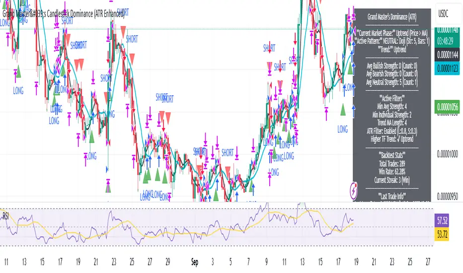
AI Volume-KNN SuperTrend - by Trading Pine Lab🇬🇧 English
The AI Volume-KNN SuperTrend is an advanced trading strategy that combines the robustness of the SuperTrend indicator with a machine-learning inspired KNN (K-Nearest Neighbors) model. The baseline is built from a volume-weighted moving average with ATR-based bands, while the KNN classifier validates trend direction in real time. This dual-layer approach reduces false signals and improves trend confirmation.
Entries are triggered when the SuperTrend flips direction and the KNN classifier confirms the move as bullish or bearish. Exits are managed with a dynamic trailing stop, automatically adjusting to SuperTrend ± ATR × factor. The strategy includes visual markers for AI start/continuation signals, as well as customizable coloring for bullish, bearish, and neutral phases.
All parameters are fully configurable:
-Trading direction filter: Long / Short / Both.
-KNN settings: number of neighbors (K), dataset size (N).
-Label smoothing: price and SuperTrend smoothing lengths (WMAs).
-SuperTrend settings: length, ATR factor, and moving average source.
-Visualization: trend markers and per-trend coloring.

FVG Ultra Assertive - Individual Filters (mtbr)FVG Ultra Assertive - Individual Filters (mtbr)
What this script offers:
This strategy detects and highlights FVGs (Fair Value Gaps) on the chart, providing traders with a visual and systematic approach to identify potential price inefficiencies. The script plots bullish and bearish FVG zones using customizable boxes and labels, allowing users to easily spot high-probability trading areas. In addition, it opens and closes simulated trades based on the detected FVGs, enabling full backtesting and strategy performance evaluation. It integrates multiple independent filters to validate the strength of each FVG signal before entering a trade.
How it works:
The script identifies:
Bullish FVGs when the current low is higher than the high of two bars ago.
Bearish FVGs when the current high is lower than the low of two bars ago.
Once an FVG is detected, it applies three optional independent filters:
GAP/ATR Filter:
Measures the FVG size relative to the Average True Range (ATR). Only gaps exceeding a user-defined multiple of ATR are considered valid.
Support/Resistance (S/R) Filter:
Uses pivot points to check if the FVG overlaps with recent high/low pivot levels within a tolerance percentage. This ensures the gap aligns with meaningful market levels.
Stochastic Filter:
Applies a stochastic oscillator to confirm momentum. Bullish FVGs are validated when stochastic values are oversold, and bearish FVGs when overbought.
After passing the selected filters, the strategy opens trades:
LONG FVG for bullish signals (buy)
SHORT FVG for bearish signals (sell)
The strategy automatically closes positions when an opposite signal appears, generating a backtest report with trades, profits, and statistics. The final bullish or bearish FVG signals are plotted as colored boxes on the chart with labels “BULL FVG” or “BEAR FVG” for immediate visual reference.
How to configure it for use:
Use GAP/ATR Filter: Enable or disable the ATR-based filter and adjust the ATR period (ATR Length) and minimum gap multiplier (Minimum Gap x ATR).
Use S/R Filter: Enable or disable the pivot-based S/R filter. Configure the pivot lookback periods (Pivot Left and Pivot Right) and the tolerance percentage (Gap Tolerance %).
Use Stochastic Filter: Enable or disable stochastic confirmation. Adjust the K and D lengths (Stoch K Length and Stoch D Length) and the overbought/oversold thresholds (Stoch Overbought and Stoch Oversold).
Colors: Customize the colors for bullish and bearish FVGs (FVG Bull and FVG Bear) to match your chart preferences.
Usage Tips:
Apply this strategy to any timeframe; shorter timeframes generate more frequent FVGs, while higher timeframes highlight stronger gaps.
Combine FVG signals with other technical analysis tools for better trade confirmation.
Use the box and label visualization to quickly scan charts for trade opportunities without cluttering the chart.
The strategy’s trades (LONG and SHORT) provide backtesting results and performance statistics for each signal.
RSI Bands With RSI - ATR Trend StrategyRSI Bands With RSI-ATR Trend Line Strategy
Overview
A trend-following strategy that combines RSI regime detection with a smoothed baseline and ATR bands. Works similar to Supertrend: the line flips bullish or bearish only when price closes beyond the band, aiming to filter noise and catch clean moves.
How It Works
RSI above 50 = bullish bias, below 50 = bearish bias
A dynamic baseline is calculated from RSI and price range, then smoothed
ATR bands expand/contract with volatility
Close above the upper band → bullish flip → long entry
Close below the lower band → bearish flip → short entry
Between bands → prior trend continues
Features
Automatic Buy/Sell entries on confirmed flips
Configurable RSI, Smoothing, ATR, and Multiplier inputs
Visual trend line (green = bull, red = bear)
Backtest ready with initial capital and commission settings
Best Use Cases
Trending markets across Forex, Crypto, Indices, Commodities
Works on multiple timeframes (higher TFs = cleaner flips)
Flexible settings for conservative swing trading or aggressive scalping
⚠️ For testing/education only. Always manage risk and confirm with higher-timeframe or structure filters.
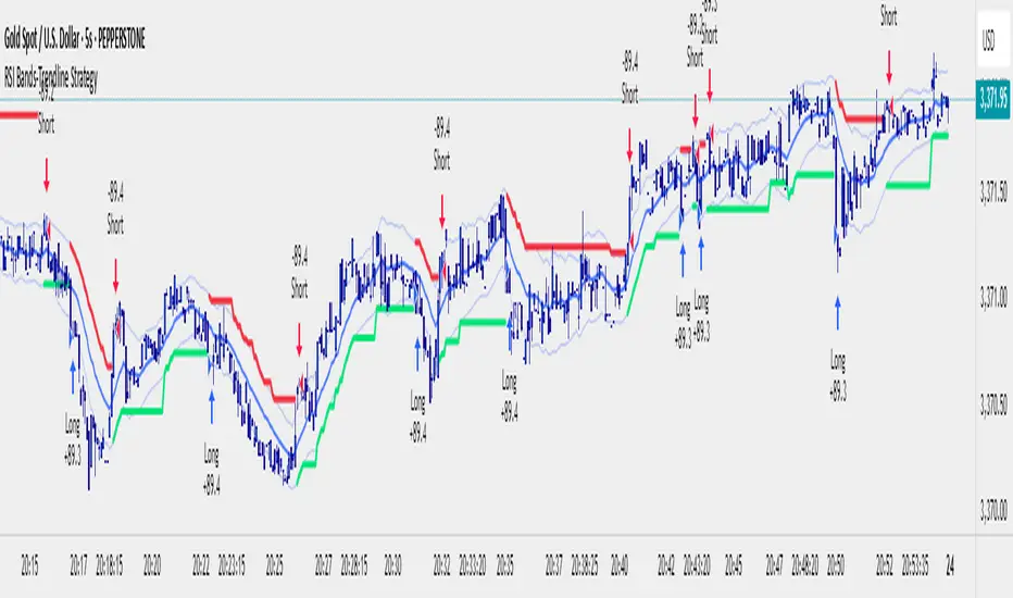
Imbalance No SL📊 Strategy Name: Imbalance No SL
This strategy specially trades on price jumps (true imbalances) in the market, takes advantage of momentum only, and as soon as the opposite signal and profit is received, the trade is closed immediately.
Imbalance No SL strategy specially generates buy and sell signals based on "Imbalance" logic, without any fixed Stop Loss.
🔍 Core Logic
Imbalance Detection
Bullish Imbalance : When the low of the current candle is above the high of the previous candle.
(i.e. a jump type gap occurred in the market – demand is high, price went straight up)
Bearish Imbalance : When the high of the current candle is below the low of the previous candle.
(i.e. the market suddenly fell down)
Creating Visual Box and Label on Signal:
As soon as bullish imbalance is found, green box & IMB BULL label is displayed on the chart.
Bearish has red box & IMB BEAR label.
Trade Entry Logic
BUY on Bullish Imbalance: If there is already a buy or neutral position, then a new “BUY” signal will fire.
SELL on Bearish Imbalance: If already in sell or neutral position, then new “SELL” signal will fire.
You can set quantity/lot size from ‘qty’ input field.
Trade Average Calculation
Buy/Sell maintains average price and their count (so that if averaging is done then correct P&L is calculated).
Trade Exit Logic (Profit Booking/Signal Reverse)
If your buy is going on and bearish imbalance is formed + price is above your average, then buy will be closed (profit condition).
If sell is going on and bullish imbalance is formed + price is below average, then sell will be closed.
Chart Cleaning/Management
Only keep the label and box of the latest signal on the chart, old boxes/labels are automatically deleted.
Alert
You can get alert on bullish or bearish signal (by using alert feature of TradingView).
✅ Simple Explanation for User
This strategy buys or sells directly at the gap (imbalance).
Whenever there is a clear signal of momentum in the market (breakout of the gap), then the trade entry takes place.
When there is an imbalance in the opposite direction and profit is made, the system closes the trade (closes).
There is no fixed stop-loss, risk management is handled by trade averaging/close.
You will know at every point on the visually chart that at which bar the buy, sell and exit took place.
⚠️ What to remember?
If the market is in trend then this script gives very good signals.
In choppy/sideways market, some loss trades can also come because there is no SL.
Big profit or big loss – both depend on the imbalance signal and market speed.

Scalping Line Strategy📌 Scalping Line Strategy – A Precision Crossover System
🔎 Overview
The Scalping Line Strategy is a short-term trading system built around the concept of momentum-driven crossovers between a smoothed moving average filter and a fast signal line. It is designed for scalpers and intraday traders who seek clear entry signals, minimal lag, and adaptive filtering to fit volatile market conditions.
At its core, the strategy uses a custom signal line ("Scalping Line"), which is derived from the difference between a double-smoothed moving average and a shorter-period signal line. Trade entries are triggered when this Scalping Line crosses above or below zero, providing a clean and rules-based framework for both long and short setups.
⚙️ Core Logic
Main Trend Filter – A double-smoothed moving average is calculated over a configurable period (default 100). This reduces noise and provides a more robust backbone for scalping signals.
Percent-Based Filter – To avoid false signals, a customizable percentage filter adjusts how closely the system “respects” price deviations from the moving average. This helps filter out insignificant fluctuations.
Signal Line – A shorter-period simple moving average (default 7) provides faster responsiveness to recent price action.
Scalping Line (SLI) – Calculated as the difference between the fast signal line and the smoothed moving average. When the SLI crosses zero, it signals a potential momentum shift.
SLI > 0 → Momentum bias is bullish.
SLI < 0 → Momentum bias is bearish.
🎯 Trade Direction & Flexibility
Trade Direction Control:
Choose between Long Only, Short Only, or Both to tailor the system to your trading style.
Signal Flip Option:
By default, long entries occur when the SLI crosses below zero, and shorts when it crosses above zero. This orientation can be flipped, allowing for alternative interpretations of the signals depending on how you want to capture momentum in your market.
🕒 Time Window Filtering
For intraday traders, a time filter can be enabled to restrict signals to specific trading sessions (e.g., 9 AM – 4 PM EST). This is particularly useful when trading assets such as equities or futures that have strong intraday volatility windows.
📈 Visuals & Clarity
Scalping Line Plot: Displayed as a dynamic oscillator around a zero baseline.
Histogram Fill: Green when above zero (bullish bias), red when below zero (bearish bias).
Signal Markers: Clear arrows mark long and short entries at crossover points.
Zero Line Reference: A flat gray line at zero assists in visually gauging momentum shifts.
🚀 Strategy Execution
Long Entry: Triggered when SLI crosses below zero (or above zero if flip is enabled) within allowed session hours.
Short Entry: Triggered when SLI crosses above zero (or below zero if flip is enabled) within allowed session hours.
Built-in Signal Cancels: Pending entries are canceled if conditions are no longer valid, ensuring no stale trades remain active.
✅ Best Use Cases
Markets: Works across equities, forex, crypto, and futures with sufficient intraday volatility.
Timeframes: Most effective on 1m to 15m charts for scalping setups, but adaptable to higher frames for swing trading.
Style: Traders who appreciate simple, rules-based momentum crossovers will find this system easy to follow and highly adaptable.
⚠️ Risk Management Note
This strategy is strictly an entry signal framework. Position sizing, stop-loss, and take-profit rules must be overlaid based on your risk management style. Always validate results with backtesting and forward testing before applying to live trading accounts.
📜 Final Thoughts
The Scalping Line Strategy offers a refined, easy-to-interpret approach to intraday trading. By combining smoothed moving averages, adaptive filtering, and flexible signal options, it helps traders identify short-term momentum shifts with clarity and confidence, making it a highly configurable tool for scalping-focused strategies.

Engulfing & Pin Bar Breakout StrategyOverview
This strategy automates a classic, powerful trading methodology based on identifying key candlestick reversal patterns and trading the subsequent price breakout. It is designed to be a complete, "set-and-go" system with built-in risk and position size management.
The core logic operates on the 1-Hour timeframe, scanning for four distinct high-probability reversal signals: two bullish and two bearish. An entry is only triggered when the market confirms the signal by breaking a key price level, aiming to capture momentum following a potential shift in market sentiment.
The Strategy Logic
The system is composed of two distinct modules: Bullish (Long) and Bearish (Short).
🐂 Bullish (Long) Setup
The script initiates a long trade based on the following strict criteria:
Signal: Identifies either a Hammer or a Bullish Engulfing pattern. These patterns often indicate that sellers are losing control and buyers are stepping in.
Confirmation: Waits for the very next candle after the signal.
Entry Trigger: A long position is automatically opened as soon as the price breaks above the high of the signal candle.
Stop Loss: Immediately set just below the low of the signal candle.
Take Profit: A fixed target is placed at a 1:5 Risk/Reward Ratio.
🐻 Bearish (Short) Setup
The script initiates a short trade based on the following strict criteria:
Signal: Identifies either a Shooting Star or a Bearish Engulfing pattern. These patterns suggest buying pressure is fading and sellers are taking over.
Confirmation: Waits for the very next candle after the signal.
Entry Trigger: A short position is automatically opened as soon as the price breaks below the low of the signal candle.
Stop Loss: Immediately set just above the high of the signal candle.
Take Profit: A fixed target is placed at a 1:4 Risk/Reward Ratio.
Key Feature: Automated Risk Management
This strategy is designed for disciplined trading. You do not need to calculate position sizes manually.
Fixed Risk: The script automatically calculates the correct position size to risk exactly 2% of your total account equity on every single trade.
Dynamic Sizing: The position size will adjust based on the distance between your entry price and your stop loss for each specific setup, ensuring a consistent risk profile.
How To Use
Apply the script to your chosen chart (e.g., BTC/USD).
Crucially, set your chart's timeframe to 1-Hour (H1). The strategy is specifically calibrated for this interval.
Navigate to the "Strategy Tester" tab below your chart to view backtest results, including net profit, win rate, and individual trades.
Disclaimer: This script is provided for educational and informational purposes only. It is not financial advice. All trading involves substantial risk, and past performance is not indicative of future results. Please use this tool responsibly and at your own risk.

Mutanabby_AI | Algo Pro Strategy# Mutanabby_AI | Algo Pro Strategy: Advanced Candlestick Pattern Trading System
## Strategy Overview
The Mutanabby_AI Algo Pro Strategy represents a systematic approach to automated trading based on advanced candlestick pattern recognition and multi-layered technical filtering. This strategy transforms traditional engulfing pattern analysis into a comprehensive trading system with sophisticated risk management and flexible position sizing capabilities.
The strategy operates on a long-only basis, entering positions when bullish engulfing patterns meet specific technical criteria and exiting when bearish engulfing patterns indicate potential trend reversals. The system incorporates multiple confirmation layers to enhance signal reliability while providing comprehensive customization options for different trading approaches and risk management preferences.
## Core Algorithm Architecture
The strategy foundation relies on bullish and bearish engulfing candlestick pattern recognition enhanced through technical analysis filtering mechanisms. Entry signals require simultaneous satisfaction of four distinct criteria: confirmed bullish engulfing pattern formation, candle stability analysis indicating decisive price action, RSI momentum confirmation below specified thresholds, and price decline verification over adjustable lookback periods.
The candle stability index measures the ratio between candlestick body size and total range including wicks, ensuring only well-formed patterns with clear directional conviction generate trading signals. This filtering mechanism eliminates indecisive market conditions where pattern reliability diminishes significantly.
RSI integration provides momentum confirmation by requiring oversold conditions before entry signal generation, ensuring alignment between pattern formation and underlying momentum characteristics. The RSI threshold remains fully adjustable to accommodate different market conditions and volatility environments.
Price decline verification examines whether current prices have decreased over a specified period, confirming that bullish engulfing patterns occur after meaningful downward movement rather than during sideways consolidation phases. This requirement enhances the probability of successful reversal pattern completion.
## Advanced Position Management System
The strategy incorporates dual position sizing methodologies to accommodate different account sizes and risk management approaches. Percentage-based position sizing calculates trade quantities as equity percentages, enabling consistent risk exposure across varying account balances and market conditions. This approach proves particularly valuable for systematic trading approaches and portfolio management applications.
Fixed quantity sizing provides precise control over trade sizes independent of account equity fluctuations, offering predictable position management for specific trading strategies or when implementing precise risk allocation models. The system enables seamless switching between sizing methods through simple configuration adjustments.
Position quantity calculations integrate seamlessly with TradingView's strategy testing framework, ensuring accurate backtesting results and realistic performance evaluation across different market conditions and time periods. The implementation maintains consistency between historical testing and live trading applications.
## Comprehensive Risk Management Framework
The strategy features dual stop loss methodologies addressing different risk management philosophies and market analysis approaches. Entry price-based stop losses calculate stop levels as fixed percentages below entry prices, providing predictable risk exposure and consistent risk-reward ratio maintenance across all trades.
The percentage-based stop loss system enables precise risk control by limiting maximum loss per trade to predetermined levels regardless of market volatility or entry timing. This approach proves essential for systematic trading strategies requiring consistent risk parameters and capital preservation during adverse market conditions.
Lowest low-based stop losses identify recent price support levels by analyzing minimum prices over adjustable lookback periods, placing stops below these technical levels with additional buffer percentages. This methodology aligns stop placement with market structure rather than arbitrary percentage calculations, potentially improving stop loss effectiveness during normal market fluctuations.
The lookback period adjustment enables optimization for different timeframes and market characteristics, with shorter periods providing tighter stops for active trading and longer periods offering broader stops suitable for position trading approaches. Buffer percentage additions ensure stops remain below obvious support levels where other market participants might place similar orders.
## Visual Customization and Interface Design
The strategy provides comprehensive visual customization through eight predefined color schemes designed for different chart backgrounds and personal preferences. Color scheme options include Classic bright green and red combinations, Ocean themes featuring blue and orange contrasts, Sunset combinations using gold and crimson, and Neon schemes providing high visibility through bright color selections.
Professional color schemes such as Forest, Royal, and Fire themes offer sophisticated alternatives suitable for business presentations and professional trading environments. The Custom color scheme enables precise color selection through individual color picker controls, maintaining maximum flexibility for specific visual requirements.
Label styling options accommodate different chart analysis preferences through text bubble, triangle, and arrow display formats. Size adjustments range from tiny through huge settings, ensuring appropriate visual scaling across different screen resolutions and chart configurations. Text color customization maintains readability across various chart themes and background selections.
## Signal Quality Enhancement Features
The strategy incorporates signal filtering mechanisms designed to eliminate repetitive signal generation during choppy market conditions. The disable repeating signals option prevents consecutive identical signals until opposing conditions occur, reducing overtrading during consolidation phases and improving overall signal quality.
Signal confirmation requirements ensure all technical criteria align before trade execution, reducing false signal occurrence while maintaining reasonable trading frequency for active strategies. The multi-layered approach balances signal quality against opportunity frequency through adjustable parameter optimization.
Entry and exit visualization provides clear trade identification through customizable labels positioned at relevant price levels. Stop loss visualization displays active risk levels through colored line plots, ensuring complete transparency regarding current risk management parameters during live trading operations.
## Implementation Guidelines and Optimization
The strategy performs effectively across multiple timeframes with optimal results typically occurring on intermediate timeframes ranging from fifteen minutes through four hours. Higher timeframes provide more reliable pattern formation and reduced false signal occurrence, while lower timeframes increase trading frequency at the expense of some signal reliability.
Parameter optimization should focus on RSI threshold adjustments based on market volatility characteristics and candlestick pattern timeframe analysis. Higher RSI thresholds generate fewer but potentially higher quality signals, while lower thresholds increase signal frequency with corresponding reliability considerations.
Stop loss method selection depends on trading style preferences and market analysis philosophy. Entry price-based stops suit systematic approaches requiring consistent risk parameters, while lowest low-based stops align with technical analysis methodologies emphasizing market structure recognition.
## Performance Considerations and Risk Disclosure
The strategy operates exclusively on long positions, making it unsuitable for bear market conditions or extended downtrend periods. Users should consider market environment analysis and broader trend assessment before implementing the strategy during adverse market conditions.
Candlestick pattern reliability varies significantly across different market conditions, with higher reliability typically occurring during trending markets compared to ranging or volatile conditions. Strategy performance may deteriorate during periods of reduced pattern effectiveness or increased market noise.
Risk management through stop loss implementation remains essential for capital preservation during adverse market movements. The strategy does not guarantee profitable outcomes and requires proper position sizing and risk management to prevent significant capital loss during unfavorable trading periods.
## Technical Specifications
The strategy utilizes standard TradingView Pine Script functions ensuring compatibility across all supported instruments and timeframes. Default configuration employs 14-period RSI calculations, adjustable candle stability thresholds, and customizable price decline verification periods optimized for general market conditions.
Initial capital settings default to $10,000 with percentage-based equity allocation, though users can adjust these parameters based on account size and risk tolerance requirements. The strategy maintains detailed trade logs and performance metrics through TradingView's integrated backtesting framework.
Alert integration enables real-time notification of entry and exit signals, stop loss executions, and other significant trading events. The comprehensive alert system supports automated trading applications and manual trade management approaches through detailed signal information provision.
## Conclusion
The Mutanabby_AI Algo Pro Strategy provides a systematic framework for candlestick pattern trading with comprehensive risk management and position sizing flexibility. The strategy's strength lies in its multi-layered confirmation approach and sophisticated customization options, enabling adaptation to various trading styles and market conditions.
Successful implementation requires understanding of candlestick pattern analysis principles and appropriate parameter optimization for specific market characteristics. The strategy serves traders seeking automated execution of proven technical analysis techniques while maintaining comprehensive control over risk management and position sizing methodologies.

Breakouts With DXY Filter Strategy [LuciTech]This advanced breakout strategy combines pivot-based breakout detection with an innovative DXY (US Dollar Index) inverse correlation filter to enhance trade selection quality. The strategy identifies breakouts from recent pivot highs and lows while using DXY movements as a confirmation filter, based on the principle that USD strength/weakness often inversely correlates with other asset movements.
Key Features
Core Breakout Logic
- Pivot-Based Detection: Identifies breakouts above recent pivot highs (bullish) and below recent pivot lows (bearish)
- Customizable Lookback: Adjustable pivot length for different market conditions
- Visual Breakout Lines: Optional display of breakout levels with customizable colors
DXY Inverse Correlation Filter
- Smart USD Filter: Uses DXY movements to confirm breakout signals
- Inverse Logic: Long signals require DXY bearishness, short signals require DXY bullishness
- Threshold Control: Minimum DXY movement percentage required for signal confirmation
- Real-time DXY Data: Pulls live DXY data for accurate correlation analysis
Moving Average Filter
- Multiple MA Types: Support for SMA, EMA, WMA, VWMA, and HMA
- Trend Confirmation: Only takes trades in the direction of the selected moving average
- Customizable Parameters: Adjustable length and source for the moving average
Advanced Risk Management
- Multiple Stop Loss Types:
- ATR-based stops with customizable multiplier
- Candle-based stops using previous candle levels
- Fixed point-based stops
- Risk-Reward Optimization: Configurable risk-reward ratios (1:1 to 1:10)
- Breakeven Function: Automatic stop loss adjustment to breakeven after specified R-multiple
- Position Sizing: Percentage-based risk management with automatic position calculation
Time-Based Trading
- Session Filter: Trade only during specified time windows
- London Time Zone: Uses Europe/London timezone for consistency
- Visual Session Highlighting: Optional background fill for active trading hours
Alert System
- Webhook Integration: JSON-formatted alerts for automated trading
- Telegram Support: Pre-formatted messages for Telegram bot integration
- Multiple Formats: Standard, Telegram, and Concise Telegram alert options
- Real-time Notifications: Instant alerts on breakout signals
How It Works
1. Breakout Detection: The script continuously monitors for closes above recent pivot highs or below recent pivot lows
2. DXY Confirmation: When a breakout occurs, the script checks if DXY is moving in the opposite direction with sufficient momentum
3. MA Filter: If enabled, ensures the breakout aligns with the overall trend direction
4. Time Filter: Validates that the signal occurs within the specified trading hours
5. Risk Calculation: Automatically calculates position size based on the defined risk percentage and stop loss distance
6. Trade Execution: Places trades with predetermined stop loss and take profit levels
Unique Advantages
- Multi-Timeframe Approach: Combines asset-specific breakouts with broader USD market sentiment
- False Breakout Reduction: DXY filter helps eliminate breakouts that lack fundamental backing
- Comprehensive Risk Management: Multiple stop loss methods and automatic position sizing
- High Customization: Extensive parameters for different trading styles and market conditions
- Professional Alert System: Ready for automated trading integration
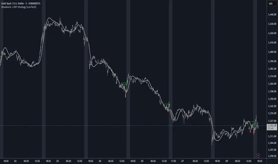
OBV ATR Strategy (OBV Breakout Channel) bas20230503ผมแก้ไขจาก OBV+SMA อันเดิม ของเดิม ดูที่เส้น SMA สองเส้นตัดกันมั่นห่วยแตกสำหรับที่ผมลองเทรดจริง และหลักการเบรค ได้แรงบันดาลใจ ATR จาก เทพคอย ที่ใช้กับราคา แต่นี้ใช้กับ OBV แทน
และผมใช้เจมินี้ เพื่อแก้ ให้ เป็น strategy เพื่อเช็คย้อนหลังได้ง่ายกว่าเดิม
หลักการง่ายคือถ้ามันขึ้น มันจะขึ้นเรื่อยๆ
เขียน แบบสุภาพ (น่าจะอ่านได้ง่ายกว่าผมเขียน)
สคริปต์นี้ได้รับการพัฒนาต่อยอดจากแนวคิด OBV+SMA Crossover แบบดั้งเดิม ซึ่งจากการทดสอบส่วนตัวพบว่าประสิทธิภาพยังไม่น่าพอใจ กลยุทธ์ใหม่นี้จึงเปลี่ยนมาใช้หลักการ "Breakout" ซึ่งได้รับแรงบันดาลใจมาจากการใช้ ATR สร้างกรอบของราคา แต่เราได้นำมาประยุกต์ใช้กับ On-Balance Volume (OBV) แทน นอกจากนี้ สคริปต์ได้ถูกแปลงเป็น Strategy เต็มรูปแบบ (โดยความช่วยเหลือจาก Gemini AI) เพื่อให้สามารถทดสอบย้อนหลัง (Backtest) และประเมินประสิทธิภาพได้อย่างแม่นยำ
หลักการของกลยุทธ์: กลยุทธ์นี้ทำงานบนแนวคิดโมเมนตัมที่ว่า "เมื่อแนวโน้มได้เกิดขึ้นแล้ว มีโอกาสที่มันจะดำเนินต่อไป" โดยจะมองหาการทะลุของพลังซื้อ-ขาย (OBV) ที่แข็งแกร่งเป็นพิเศษเป็นสัญญาณเข้าเทร
----
สคริปต์นี้เป็นกลยุทธ์ (Strategy) ที่ใช้ On-Balance Volume (OBV) ซึ่งเป็นอินดิเคเตอร์ที่วัดแรงซื้อและแรงขายสะสม แทนที่จะใช้การตัดกันของเส้นค่าเฉลี่ย (SMA Crossover) ที่เป็นแบบพื้นฐาน กลยุทธ์นี้จะมองหาการ "ทะลุ" (Breakout) ของพลัง OBV ออกจากกรอบสูงสุด-ต่ำสุดของตัวเองในรอบที่ผ่านมา
สัญญาณกระทิง (Bull Signal): เกิดขึ้นเมื่อพลังการซื้อ (OBV) แข็งแกร่งจนสามารถทะลุจุดสูงสุดของตัวเองในอดีตได้ บ่งบอกถึงโอกาสที่แนวโน้มจะเปลี่ยนเป็นขาขึ้น
สัญญาณหมี (Bear Signal): เกิดขึ้นเมื่อพลังการขาย (OBV) รุนแรงจนสามารถกดดันให้ OBV ทะลุจุดต่ำสุดของตัวเองในอดีตได้ บ่งบอกถึงโอกาสที่แนวโน้มจะเปลี่ยนเป็นขาลง
ส่วนประกอบบนกราฟ (Indicator Components)
เส้น OBV
เส้นหลัก ที่เปลี่ยนเขียวเป็นแดง เป็นทั้งแนวรับและแนวต้าน และ จุด stop loss
เส้นนี้คือหัวใจของอินดิเคเตอร์ ที่แสดงถึงพลังสะสมของ Volume
เมื่อเส้นเป็นสีเขียว (แนวรับ): จะปรากฏขึ้นเมื่อกลยุทธ์เข้าสู่ "โหมดกระทิง" เส้นนี้คือระดับต่ำสุดของ OBV ในอดีต และทำหน้าที่เป็นแนวรับไดนามิก
เมื่อเส้นกลายเป็นสีแดงสีแดง (แนวต้าน): จะปรากฏขึ้นเมื่อกลยุทธ์เข้าสู่ "โหมดหมี" เส้นนี้คือระดับสูงสุดของ OBV ในอดีต และทำหน้าที่เป็นแนวต้านไดนามิก
สัญลักษณ์สัญญาณ (Signal Markers):
Bull 🔼 (สามเหลี่ยมขึ้นสีเขียว): คือสัญญาณ "เข้าซื้อ" (Long) จะปรากฏขึ้น ณ จุดที่ OBV ทะลุขึ้นไปเหนือกรอบด้านบนเป็นครั้งแรก
Bear 🔽 (สามเหลี่ยมลงสีแดง): คือสัญญาณ "เข้าขาย" (Short) จะปรากฏขึ้น ณ จุดที่ OBV ทะลุลงไปต่ำกว่ากรอบด้านล่างเป็นครั้งแรก
วิธีการใช้งาน (How to Use)
เพิ่มสคริปต์นี้ลงบนกราฟราคาที่คุณสนใจ
ไปที่แท็บ "Strategy Tester" ด้านล่างของ TradingView เพื่อดูผลการทดสอบย้อนหลัง (Backtest) ของกลยุทธ์บนสินทรัพย์และไทม์เฟรมต่างๆ
ใช้สัญลักษณ์ "Bull" และ "Bear" เป็นตัวช่วยในการตัดสินใจเข้าเทรด
ข้อควรจำ: ไม่มีกลยุทธ์ใดที่สมบูรณ์แบบ 100% ควรใช้สคริปต์นี้ร่วมกับการวิเคราะห์ปัจจัยอื่นๆ เช่น โครงสร้างราคา, แนวรับ-แนวต้านของราคา และการบริหารความเสี่ยง (Risk Management) ของตัวคุณเองเสมอ
การตั้งค่า (Inputs)
SMA Length 1 / SMA Length 2: ใช้สำหรับพล็อตเส้นค่าเฉลี่ยของ OBV เพื่อดูเป็นภาพอ้างอิง ไม่มีผลต่อตรรกะการเข้า-ออกของ Strategy อันใหม่ แต่มันเป็นของเก่า ถ้าชอบ ก็ใช้ได้ เมื่อ SMA สองเส้นตัดกัน หรือตัดกับเส้น OBV
High/Low Lookback Length: (ค่าพื้นฐาน30/แก้ตรงนี้ให้เหมาะสมกับ coin หรือหุ้น ตามความผันผวน ) คือระยะเวลาที่ใช้ในการคำนวณกรอบสูงสุด-ต่ำสุดของ OBV
ค่าน้อย: ทำให้กรอบแคบลง สัญญาณจะเกิดไวและบ่อยขึ้น แต่อาจมีสัญญาณหลอก (False Signal) เยอะขึ้น
ค่ามาก: ทำให้กรอบกว้างขึ้น สัญญาณจะเกิดช้าลงและน้อยลง แต่มีแนวโน้มที่จะเป็นสัญญาณที่แข็งแกร่งกว่า
แน่นอนครับ นี่คือคำแปลฉบับภาษาอังกฤษที่สรุปใจความสำคัญ กระชับ และสุภาพ เหมาะสำหรับนำไปใช้ในคำอธิบายสคริปต์ (Description) ของ TradingView ครับ
---Translate to English---
OBV Breakout Channel Strategy
This script is an evolution of a traditional OBV+SMA Crossover concept. Through personal testing, the original crossover method was found to have unsatisfactory performance. This new strategy, therefore, uses a "Breakout" principle. The inspiration comes from using ATR to create price channels, but this concept has been adapted and applied to On-Balance Volume (OBV) instead.
Furthermore, the script has been converted into a full Strategy (with assistance from Gemini AI) to enable precise backtesting and performance evaluation.
The strategy's core principle is momentum-based: "once a trend is established, it is likely to continue." It seeks to enter trades on exceptionally strong breakouts of buying or selling pressure as measured by OBV.
Core Concept
This is a Strategy that uses On-Balance Volume (OBV), an indicator that measures cumulative buying and selling pressure. Instead of relying on a basic Simple Moving Average (SMA) Crossover, this strategy identifies a "Breakout" of the OBV from its own highest-high and lowest-low channel over a recent period.
Bull Signal: Occurs when the buying pressure (OBV) is strong enough to break above its own recent highest high, indicating a potential shift to an upward trend.
Bear Signal: Occurs when the selling pressure (OBV) is intense enough to push the OBV below its own recent lowest low, indicating a potential shift to a downward trend.
On-Screen Components
1. OBV Line
This is the main indicator line, representing the cumulative volume. Its color changes to green when OBV is rising and red when it is falling.
2. Dynamic Support & Resistance Line
This is the thick Green or Red line that appears based on the strategy's current "mode." This line serves as a dynamic support/resistance level and can be used as a reference for stop-loss placement.
Green Line (Support): Appears when the strategy enters "Bull Mode." This line represents the lowest low of the OBV in the recent past and acts as dynamic support.
Red Line (Resistance): Appears when the strategy enters "Bear Mode." This line represents the highest high of the OBV in the recent past and acts as dynamic resistance.
3. Signal Markers
Bull 🔼 (Green Up Triangle): This is the "Long Entry" signal. It appears at the moment the OBV first breaks out above its high-low channel.
Bear 🔽 (Red Down Triangle): This is the "Short Entry" signal. It appears at the moment the OBV first breaks down below its high-low channel.
How to Use
Add this script to the price chart of your choice.
Navigate to the "Strategy Tester" panel at the bottom of TradingView to view the backtesting results for the strategy on different assets and timeframes.
Use the "Bull" and "Bear" signals as aids in your trading decisions.
Disclaimer: No strategy is 100% perfect. This script should always be used in conjunction with other forms of analysis, such as price structure, key price-based support/resistance levels, and your own personal risk management rules.
Inputs
SMA Length 1 / SMA Length 2: These are used to plot moving averages on the OBV for visual reference. They are part of the legacy logic and do not affect the new breakout strategy. However, they are kept for traders who may wish to observe their crossovers for additional confirmation.
High/Low Lookback Length: (Most Important Setting) This determines the period used to calculate the highest-high and lowest-low OBV channel. (Default is 30; adjust this to suit the asset's volatility).
A smaller value: Creates a narrower channel, leading to more frequent and faster signals, but potentially more false signals.
A larger value: Creates a wider channel, leading to fewer and slower signals, which are likely to be more significant.
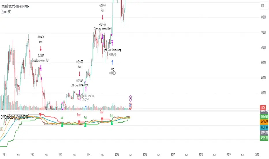
Anomalous Holonomy Field Theory🌌 Anomalous Holonomy Field Theory (AHFT) - Revolutionary Quantum Market Analysis
Where Theoretical Physics Meets Trading Reality
A Groundbreaking Synthesis of Differential Geometry, Quantum Field Theory, and Market Dynamics
🔬 THEORETICAL FOUNDATION - THE MATHEMATICS OF MARKET REALITY
The Anomalous Holonomy Field Theory represents an unprecedented fusion of advanced mathematical physics with practical market analysis. This isn't merely another indicator repackaging old concepts - it's a fundamentally new lens through which to view and understand market structure .
1. HOLONOMY GROUPS (Differential Geometry)
In differential geometry, holonomy measures how vectors change when parallel transported around closed loops in curved space. Applied to markets:
Mathematical Formula:
H = P exp(∮_C A_μ dx^μ)
Where:
P = Path ordering operator
A_μ = Market connection (price-volume gauge field)
C = Closed price path
Market Implementation:
The holonomy calculation measures how price "remembers" its journey through market space. When price returns to a previous level, the holonomy captures what has changed in the market's internal geometry. This reveals:
Hidden curvature in the market manifold
Topological obstructions to arbitrage
Geometric phase accumulated during price cycles
2. ANOMALY DETECTION (Quantum Field Theory)
Drawing from the Adler-Bell-Jackiw anomaly in quantum field theory:
Mathematical Formula:
∂_μ j^μ = (e²/16π²)F_μν F̃^μν
Where:
j^μ = Market current (order flow)
F_μν = Field strength tensor (volatility structure)
F̃^μν = Dual field strength
Market Application:
Anomalies represent symmetry breaking in market structure - moments when normal patterns fail and extraordinary opportunities arise. The system detects:
Spontaneous symmetry breaking (trend reversals)
Vacuum fluctuations (volatility clusters)
Non-perturbative effects (market crashes/melt-ups)
3. GAUGE THEORY (Theoretical Physics)
Markets exhibit gauge invariance - the fundamental physics remains unchanged under certain transformations:
Mathematical Formula:
A'_μ = A_μ + ∂_μΛ
This ensures our signals are gauge-invariant observables , immune to arbitrary market "coordinate changes" like gaps or reference point shifts.
4. TOPOLOGICAL DATA ANALYSIS
Using persistent homology and Morse theory:
Mathematical Formula:
β_k = dim(H_k(X))
Where β_k are the Betti numbers describing topological features that persist across scales.
🎯 REVOLUTIONARY SIGNAL CONFIGURATION
Signal Sensitivity (0.5-12.0, default 2.5)
Controls the responsiveness of holonomy field calculations to market conditions. This parameter directly affects the threshold for detecting quantum phase transitions in price action.
Optimization by Timeframe:
Scalping (1-5min): 1.5-3.0 for rapid signal generation
Day Trading (15min-1H): 2.5-5.0 for balanced sensitivity
Swing Trading (4H-1D): 5.0-8.0 for high-quality signals only
Score Amplifier (10-200, default 50)
Scales the raw holonomy field strength to produce meaningful signal values. Higher values amplify weak signals in low-volatility environments.
Signal Confirmation Toggle
When enabled, enforces additional technical filters (EMA and RSI alignment) to reduce false positives. Essential for conservative strategies.
Minimum Bars Between Signals (1-20, default 5)
Prevents overtrading by enforcing quantum decoherence time between signals. Higher values reduce whipsaws in choppy markets.
👑 ELITE EXECUTION SYSTEM
Execution Modes:
Conservative Mode:
Stricter signal criteria
Higher quality thresholds
Ideal for stable market conditions
Adaptive Mode:
Self-adjusting parameters
Balances signal frequency with quality
Recommended for most traders
Aggressive Mode:
Maximum signal sensitivity
Captures rapid market moves
Best for experienced traders in volatile conditions
Dynamic Position Sizing:
When enabled, the system scales position size based on:
Holonomy field strength
Current volatility regime
Recent performance metrics
Advanced Exit Management:
Implements trailing stops based on ATR and signal strength, with mode-specific multipliers for optimal profit capture.
🧠 ADAPTIVE INTELLIGENCE ENGINE
Self-Learning System:
The strategy analyzes recent trade outcomes and adjusts:
Risk multipliers based on win/loss ratios
Signal weights according to performance
Market regime detection for environmental adaptation
Learning Speed (0.05-0.3):
Controls adaptation rate. Higher values = faster learning but potentially unstable. Lower values = stable but slower adaptation.
Performance Window (20-100 trades):
Number of recent trades analyzed for adaptation. Longer windows provide stability, shorter windows increase responsiveness.
🎨 REVOLUTIONARY VISUAL SYSTEM
1. Holonomy Field Visualization
What it shows: Multi-layer quantum field bands representing market resonance zones
How to interpret:
Blue/Purple bands = Primary holonomy field (strongest resonance)
Band width = Field strength and volatility
Price within bands = Normal quantum state
Price breaking bands = Quantum phase transition
Trading application: Trade reversals at band extremes, breakouts on band violations with strong signals.
2. Quantum Portals
What they show: Entry signals with recursive depth patterns indicating momentum strength
How to interpret:
Upward triangles with portals = Long entry signals
Downward triangles with portals = Short entry signals
Portal depth = Signal strength and expected momentum
Color intensity = Probability of success
Trading application: Enter on portal appearance, with size proportional to portal depth.
3. Field Resonance Bands
What they show: Fibonacci-based harmonic price zones where quantum resonance occurs
How to interpret:
Dotted circles = Minor resonance levels
Solid circles = Major resonance levels
Color coding = Resonance strength
Trading application: Use as dynamic support/resistance, expect reactions at resonance zones.
4. Anomaly Detection Grid
What it shows: Fractal-based support/resistance with anomaly strength calculations
How to interpret:
Triple-layer lines = Major fractal levels with high anomaly probability
Labels show: Period (H8-H55), Price, and Anomaly strength (φ)
⚡ symbol = Extreme anomaly detected
● symbol = Strong anomaly
○ symbol = Normal conditions
Trading application: Expect major moves when price approaches high anomaly levels. Use for precise entry/exit timing.
5. Phase Space Flow
What it shows: Background heatmap revealing market topology and energy
How to interpret:
Dark background = Low market energy, range-bound
Purple glow = Building energy, trend developing
Bright intensity = High energy, strong directional move
Trading application: Trade aggressively in bright phases, reduce activity in dark phases.
📊 PROFESSIONAL DASHBOARD METRICS
Holonomy Field Strength (-100 to +100)
What it measures: The Wilson loop integral around price paths
>70: Strong positive curvature (bullish vortex)
<-70: Strong negative curvature (bearish collapse)
Near 0: Flat connection (range-bound)
Anomaly Level (0-100%)
What it measures: Quantum vacuum expectation deviation
>70%: Major anomaly (phase transition imminent)
30-70%: Moderate anomaly (elevated volatility)
<30%: Normal quantum fluctuations
Quantum State (-1, 0, +1)
What it measures: Market wave function collapse
+1: Bullish eigenstate |↑⟩
0: Superposition (uncertain)
-1: Bearish eigenstate |↓⟩
Signal Quality Ratings
LEGENDARY: All quantum fields aligned, maximum probability
EXCEPTIONAL: Strong holonomy with anomaly confirmation
STRONG: Good field strength, moderate anomaly
MODERATE: Decent signals, some uncertainty
WEAK: Minimal edge, high quantum noise
Performance Metrics
Win Rate: Rolling performance with emoji indicators
Daily P&L: Real-time profit tracking
Adaptive Risk: Current risk multiplier status
Market Regime: Bull/Bear classification
🏆 WHY THIS CHANGES EVERYTHING
Traditional technical analysis operates on 100-year-old principles - moving averages, support/resistance, and pattern recognition. These work because many traders use them, creating self-fulfilling prophecies.
AHFT transcends this limitation by analyzing markets through the lens of fundamental physics:
Markets have geometry - The holonomy calculations reveal this hidden structure
Price has memory - The geometric phase captures path-dependent effects
Anomalies are predictable - Quantum field theory identifies symmetry breaking
Everything is connected - Gauge theory unifies disparate market phenomena
This isn't just a new indicator - it's a new way of thinking about markets . Just as Einstein's relativity revolutionized physics beyond Newton's mechanics, AHFT revolutionizes technical analysis beyond traditional methods.
🔧 OPTIMAL SETTINGS FOR MNQ 10-MINUTE
For the Micro E-mini Nasdaq-100 on 10-minute timeframe:
Signal Sensitivity: 2.5-3.5
Score Amplifier: 50-70
Execution Mode: Adaptive
Min Bars Between: 3-5
Theme: Quantum Nebula or Dark Matter
💭 THE JOURNEY - FROM IMPOSSIBLE THEORY TO TRADING REALITY
Creating AHFT was a mathematical odyssey that pushed the boundaries of what's possible in Pine Script. The journey began with a seemingly impossible question: Could the profound mathematical structures of theoretical physics be translated into practical trading tools?
The Theoretical Challenge:
Months were spent diving deep into differential geometry textbooks, studying the works of Chern, Simons, and Witten. The mathematics of holonomy groups and gauge theory had never been applied to financial markets. Translating abstract mathematical concepts like parallel transport and fiber bundles into discrete price calculations required novel approaches and countless failed attempts.
The Computational Nightmare:
Pine Script wasn't designed for quantum field theory calculations. Implementing the Wilson loop integral, managing complex array structures for anomaly detection, and maintaining computational efficiency while calculating geometric phases pushed the language to its limits. There were moments when the entire project seemed impossible - the script would timeout, produce nonsensical results, or simply refuse to compile.
The Breakthrough Moments:
After countless sleepless nights and thousands of lines of code, breakthrough came through elegant simplifications. The realization that market anomalies follow patterns similar to quantum vacuum fluctuations led to the revolutionary anomaly detection system. The discovery that price paths exhibit holonomic memory unlocked the geometric phase calculations.
The Visual Revolution:
Creating visualizations that could represent 4-dimensional quantum fields on a 2D chart required innovative approaches. The multi-layer holonomy field, recursive quantum portals, and phase space flow representations went through dozens of iterations before achieving the perfect balance of beauty and functionality.
The Balancing Act:
Perhaps the greatest challenge was maintaining mathematical rigor while ensuring practical trading utility. Every formula had to be both theoretically sound and computationally efficient. Every visual had to be both aesthetically pleasing and information-rich.
The result is more than a strategy - it's a synthesis of pure mathematics and market reality that reveals the hidden order within apparent chaos.
📚 INTEGRATED DOCUMENTATION
Once applied to your chart, AHFT includes comprehensive tooltips on every input parameter. The source code contains detailed explanations of the mathematical theory, practical applications, and optimization guidelines. This published description provides the overview - the indicator itself is a complete educational resource.
⚠️ RISK DISCLAIMER
While AHFT employs advanced mathematical models derived from theoretical physics, markets remain inherently unpredictable. No mathematical model, regardless of sophistication, can guarantee future results. This strategy uses realistic commission ($0.62 per contract) and slippage (1 tick) in all calculations. Past performance does not guarantee future results. Always use appropriate risk management and never risk more than you can afford to lose.
🌟 CONCLUSION
The Anomalous Holonomy Field Theory represents a quantum leap in technical analysis - literally. By applying the profound insights of differential geometry, quantum field theory, and gauge theory to market analysis, AHFT reveals structure and opportunities invisible to traditional methods.
From the holonomy calculations that capture market memory to the anomaly detection that identifies phase transitions, from the adaptive intelligence that learns and evolves to the stunning visualizations that make the invisible visible, every component works in mathematical harmony.
This is more than a trading strategy. It's a new lens through which to view market reality.
Trade with the precision of physics. Trade with the power of mathematics. Trade with AHFT.
I hope this serves as a good replacement for Quantum Edge Pro - Adaptive AI until I'm able to fix it.
— Dskyz, Trade with insight. Trade with anticipation.
