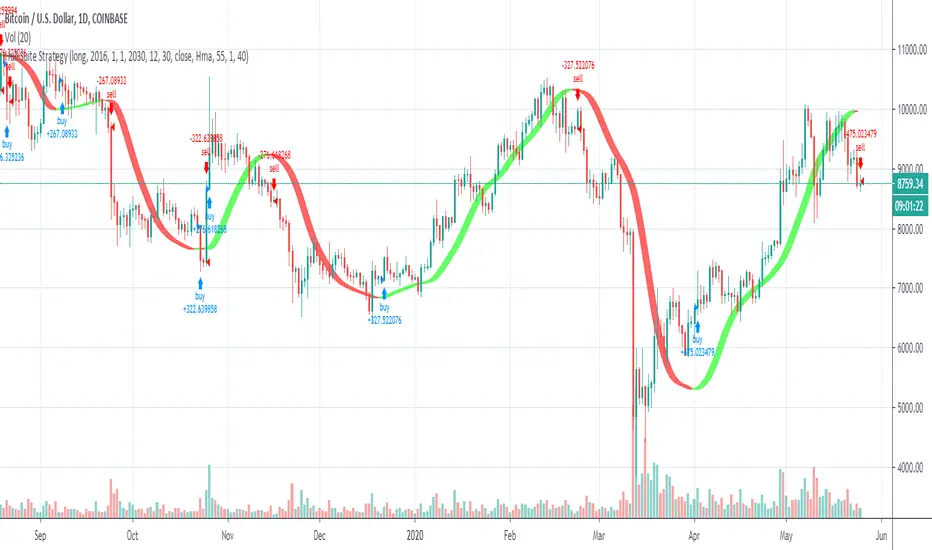
Hull Suite StrategyConverted the hull suite into a strategy script for easy backtesting and added ability to specify a time periods to backtest over.
Buscar en scripts para "backtesting"
SupterTrend I created this script for basically two reasons
1. there is not simple suptertrend indicator available on tv rather you will find many fancy suptrend indicators with confusing other indicators and absurd background colors i dont know why some of the trader coders are obsessed with is using over the top color and designing phenomena.
2. I want to let people know about the accuracy of suptertrend indicator on multiple time frames i am plaining to create a backtesting tool for almost all Famous indicators so that specially new folks know what should they expect from any particular Indicator
Also i added intraday filter to check the results for intrday signals . the sqaure off timings are for Indian markets only but you can edit the hours and minutes in the code for using other than indian markets. No need to do anything if you only want positional trading trading results

Patient Trendfollower (7)(alpha) Backtesting AlgorithmThis is an alpha version of backtesting algorithm for my Patient Trendfollower (7) strategy. It can help you adapt the indicator to other charts than EURUSD. Please bear in mind that price action, volume profiles and supzistences are a catalyst for successful trading, not an indicator. You can get significantly better results if you use these things in your trading and use Trendfollower only as a secondary tool.
Patient Trendfollower Indicator
Thanks belongs to @everget and Satik FX, their contributions are highlighted on an indicator page.

BO - RSI - M5 BacktestingBO - RSI - M5 Backtesting -Rule of Strategy
A. Data
1. Chart M5 IDC
2. Symbol: EURJPY
B. Indicator
1. RSI
2. Length: 12 (adjustable)
3. Extreme Top: 75 (adjustable)
4. Extreme Bottom: 25 (adjustable)
C. Rule of Signal
1. Put Signal
* Rsi create a temporary peak over Extreme Top
row61: peak_rsi= rsi >rsi and rsi >rsi and rsi rsi_top
2. Call Signal
* Rsi create a temporary bottom under Extreme Bottom
row62: bott_rsi= rsi rsi and rsi

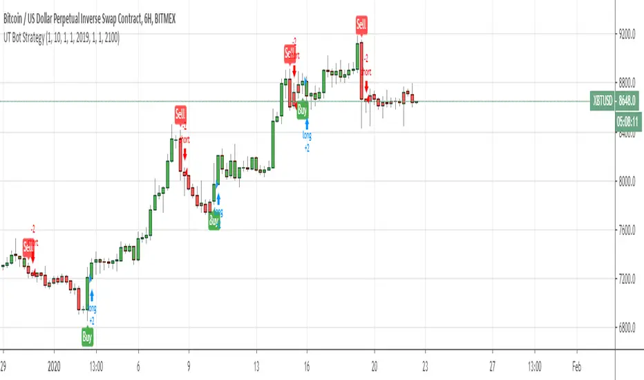
UT Bot Strategy with Backtesting Range [QuantNomad]UT Bot indicator was inially developer by @Yo_adriiiiaan
Idea of original code belongs @HPotter
I can't update my original UT Bot Strategy so I publishing new strategy with backtesting range included.
I just took code of Yo_adriiiiaan, cleaned it, deleted all useless pieces of code, transformet to v4 and created a strategy from it.
Also I added an input that allows you to swich to signals from Heiking Ashi. I saw that author uses HA for the indicator and on HA it look much nices then on real candles.
Do not add this strategy to HA candles, use usual candles and this checkbox.
Original script:
UT Bot
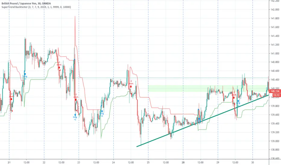
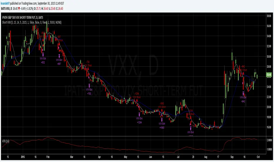
SuperTrend BacktesterThis is a backtesting script for the famous Super Trend.
Features
- Custom Date Range
- Custom Targets and Risks
Requested by Dlatrella
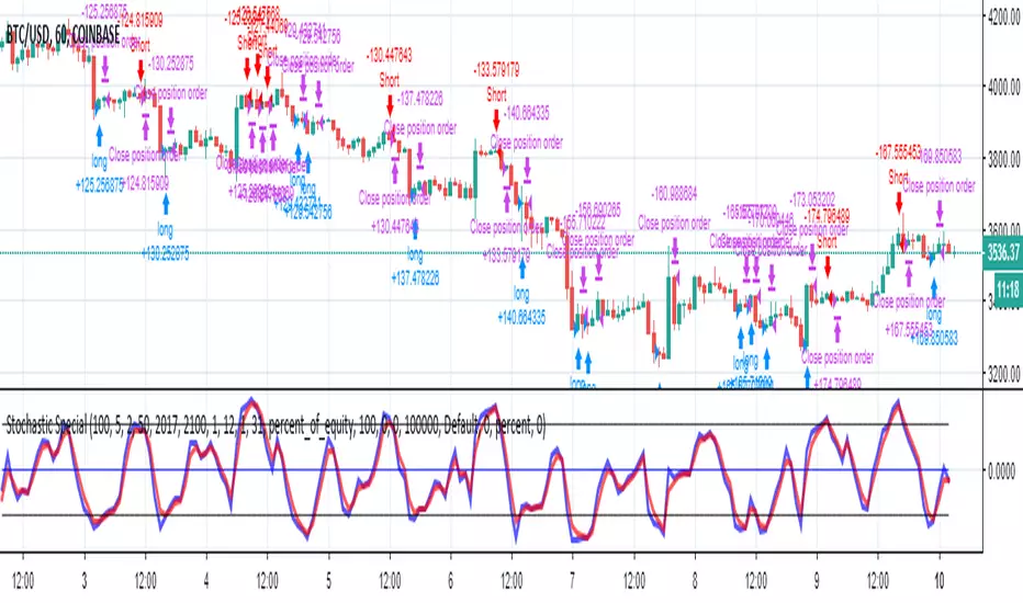
CS Basic Scripts - Stochastic Special (Strategy)This Stochastic Special Strategy features inputs for:
- Custom Backtesting Date Range
- Long and Short Strategy Discinctions
- Utilize SMI, RSI, Martingale, and Body-Filter Strategy
- Adjust the SMI Percent Lengths and Limit
- Automate with the Autoview Trading Bot
Strategy script may be tested by favoriting and adding to any chart.
Study script is available for automated trading at www.cryptoscores.org
Deviation Back Tester (Great for Credit Spreads)!Error with math fixed in this one. Please use this one.
This is great for credit spreads! Lets say you wanted to know if you had sold a 15% OTM Bull Put vertical 2 months out, how often would you win? This Turns green if you would have been correct with your credit spread had it expired on that date, or red if you would've been wrong. Great for Back testing!
This could also be used for ATM debit spreads credit spreads etc. Example, how often does SPY deviate outside a 10% range relative to two months, 5% (if your doing straddles perhaps) etc.
This Can be used with any stock.
PLEASE KEEP IN MIND THAT IT TESTS DEVIATION IN BOTH DIRECTIONS. THEREFORE IT WILL HIGHLIGHT RED ON BOTH THE UPSIDE AND DOWNSIDE. WHEN BACKTESTING BE SURE TO CHECK WHETHER IT IS RED BECAUSE OF DOWNSIDE OR UPSIDE.
Simple Candle Info This script shows the following simple information about the last candle:
- Candle size
- Body size included %
- Top Wick size
- Bottom Wick size
- Top Wick + Body size
- Bottom Wick + Body size
You can change:
- colors and position for labels
- add information for previous candle too
- change language

Laguerre RSI by KivancOzbilgic STRATEGYBacktesting.
" Laguerre RSI is based on John EHLERS' Laguerre Filter to avoid the noise of RSI .
Change alpha coefficient to increase/decrease lag and smoothness.
Buy when Laguerre RSI crosses upwards above 20.
Sell when Laguerre RSI crosses down below 80.
While indicator runs flat above 80 level, it means that an uptrend is strong.
While indicator runs flat below 20 level, it means that a downtrend is strong. "
Developer: John EHLERS
Author: KivancOzbilgic

Simple Price Momentum - How To Create A Simple Trading StrategyThis script was built using a logical approach to trading systems. All the details can be found in a step by step guide below. I hope you enjoy it. I am really glad to be part of this community. Thank you all. I hope you not only succeed on your trading career but also enjoy it.
docs.google.com
Moving Averages Cross - MTF - StrategyBacktesting Script for the following strategy
Strategy Injector Source: github.com
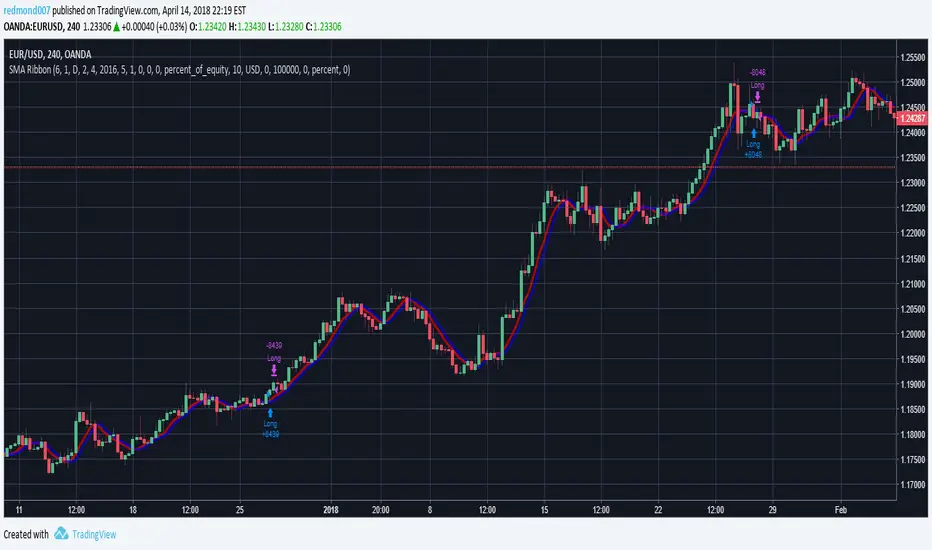
Dual Timeframe SMA Ribbon Crossover Backtest// Backtesting Dual SMA Ribbon Crossover Strategy
// see f.bpcdn.co
// including time limiting
Turned this study into a backtest.

Entropy Divergence (No Repaint) [PhenLabs]📊 Entropy Divergence (No Repaint)
Version: PineScript™ v6
📌 Description
The Entropy Divergence Scalper (EDS) is a sophisticated trading indicator that applies information theory to market analysis. By calculating Shannon Entropy on price returns, it identifies periods when market behavior becomes more predictable and orderly—the ideal conditions for divergence-based trading.
Traditional divergence indicators generate signals regardless of market conditions, leading to many false signals during chaotic, high-entropy periods. EDS solves this by acting as an intelligent filter: it only triggers signals when entropy drops below your specified threshold, indicating that the market has entered a more structured, tradeable state.
This indicator is built with a strict non-repainting guarantee. All signals use barstate.isconfirmed and only appear after bar close, giving you reliable signals you can trust for live trading.
🚀 Points of Innovation
Shannon Entropy integration measures market randomness using information theory mathematics
Dual divergence engine detects both RSI and Volume divergences simultaneously
Entropy-filtered signals eliminate noise by only triggering in low-entropy (predictable) market conditions
100% non-repainting architecture ensures all signals are confirmed and historically accurate
Multi-layer confirmation combines entropy state, RSI divergence, and volume divergence for higher probability setups
Dynamic color visualization provides instant visual feedback on current market entropy state
🔧 Core Components
Shannon Entropy Calculator: Bins price returns into histograms and calculates entropy using H(X) = -Σ p(x) × log₂(p(x))
RSI Divergence Detector: Identifies when price makes lower lows while RSI makes higher lows (bullish) or price makes higher highs while RSI makes lower highs (bearish)
Volume Divergence Detector: Spots increasing volume interest at price lows (bullish) or decreasing conviction at price highs (bearish)
Pivot Detection System: Uses configurable lookback periods to identify and track price, RSI, and volume pivots
Signal Classification Engine: Labels signals as RSI, VOL, or RSI+VOL based on which divergences triggered
🔥 Key Features
Entropy Threshold Control: Set your preferred entropy level (default 2.5) to filter out signals during chaotic market periods
Configurable Smoothing: EMA smoothing on entropy values reduces noise while maintaining signal responsiveness
Flexible Pivot Detection: Adjust left/right lookback bars to tune sensitivity for different trading styles
Divergence Search Range: Control how far back the indicator looks for divergence patterns (20-200 bars)
Minimum Pivot Distance: Prevents false signals from pivots that are too close together
Complete Alert System: Four alert conditions for bullish signals, bearish signals, any signal, and low entropy zone entry
🎨 Visualization
Dynamic Entropy Line: Color gradient shifts from green (low entropy/tradeable) to orange (high entropy/chaotic)
Entropy Threshold Line: Dashed reference line shows your configured entropy threshold
Low Entropy Zone Fill: Background highlighting indicates when market is in tradeable low-entropy state
Scaled RSI Plot: RSI overlay scaled to fit the entropy pane for easy correlation analysis
Normalized Volume Bars: Volume displayed as columns normalized against 20-period average
Signal Labels: Clear LONG/SHORT labels with divergence type (RSI, VOL, or RSI+VOL)
Information Table: Real-time display of entropy value, state, RSI, and current signal status
📖 Usage Guidelines
Entropy Lookback Period — Default: 20, Range: 5-100 — Controls how many bars are used for entropy calculation; higher values provide smoother readings but slower response
Histogram Bins — Default: 10, Range: 5-50 — Number of bins for probability distribution; more bins provide finer granularity
Low Entropy Threshold — Default: 2.5, Range: 0.5-4.0 — Signals only trigger when entropy drops below this value; lower settings are more selective
Entropy Smoothing — Default: 3, Range: 1-10 — EMA smoothing applied to raw entropy values for noise reduction
RSI Length — Default: 14, Range: 5-50 — Standard RSI calculation period
Pivot Lookback Left — Default: 5, Range: 2-20 — Bars to the left for pivot detection
Pivot Lookback Right — Default: 2, Range: 1-10 — Bars to the right for pivot confirmation; lower values produce faster signals
Divergence Search Range — Default: 60, Range: 20-200 — Maximum bars to look back for divergence comparison
Min Bars Between Pivots — Default: 5, Range: 3-30 — Minimum distance between pivots for valid divergence detection
✅ Best Use Cases
Scalping during low-volatility consolidation periods when entropy drops and price becomes more predictable
Swing trade entry timing by waiting for divergence signals in low-entropy market conditions
Trend reversal identification when both RSI and Volume divergences align with low entropy readings
Multi-timeframe confirmation by checking entropy state on higher timeframes before taking signals
Filtering existing strategies by adding entropy as a confirmation layer to reduce false signals
⚠️ Limitations
Signals appear with a delay due to pivot confirmation requirements (pivotLookbackRight bars after pivot forms)
May generate fewer signals during strongly trending markets where entropy remains elevated
Entropy threshold requires optimization for different instruments and timeframes
Not designed for high-frequency trading due to bar-close confirmation requirement
Divergences can fail in extremely strong trends where momentum overwhelms the signal
💡 What Makes This Unique
First indicator to combine Shannon Entropy filtering with multi-factor divergence detection
Information theory approach provides mathematical foundation for identifying tradeable market states
Triple confirmation requirement (low entropy + divergence + bar close) significantly reduces false signals
Non-repainting guarantee makes it suitable for strategy backtesting and live trading
Open-source PineScript v6 code allows traders to understand and customize the methodology
🔬 How It Works
Step 1 — Entropy Calculation: The indicator calculates logarithmic returns, bins them into a histogram, and computes Shannon Entropy to measure market randomness
Step 2 — Entropy Filtering: When smoothed entropy drops below the threshold, the market is considered to be in a tradeable low-entropy state
Step 3 — Pivot Detection: The system continuously tracks price, RSI, and volume pivots using configurable lookback parameters
Step 4 — Divergence Analysis: When a new pivot is confirmed, the indicator compares it against previous pivots to detect bullish or bearish divergences
Step 5 — Signal Generation: A final signal only triggers when low entropy conditions coincide with a confirmed divergence pattern on a closed bar
💡 Note:
This indicator is designed for educational purposes and technical analysis. Always use proper risk management and never risk more than you can afford to lose. The non-repainting guarantee means signals will only appear after bar close—watch the indicator in real-time to verify this behavior. For optimal results, consider combining EDS signals with support/resistance levels and overall market context.

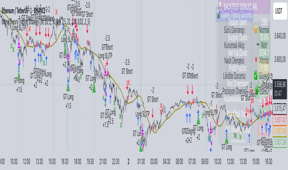
Game Theory Trading StrategyGame Theory Trading Strategy: Explanation and Working Logic
This Pine Script (version 5) code implements a trading strategy named "Game Theory Trading Strategy" in TradingView. Unlike the previous indicator, this is a full-fledged strategy with automated entry/exit rules, risk management, and backtesting capabilities. It uses Game Theory principles to analyze market behavior, focusing on herd behavior, institutional flows, liquidity traps, and Nash equilibrium to generate buy (long) and sell (short) signals. Below, I'll explain the strategy's purpose, working logic, key components, and usage tips in detail.
1. General Description
Purpose: The strategy identifies high-probability trading opportunities by combining Game Theory concepts (herd behavior, contrarian signals, Nash equilibrium) with technical analysis (RSI, volume, momentum). It aims to exploit market inefficiencies caused by retail herd behavior, institutional flows, and liquidity traps. The strategy is designed for automated trading with defined risk management (stop-loss/take-profit) and position sizing based on market conditions.
Key Features:
Herd Behavior Detection: Identifies retail panic buying/selling using RSI and volume spikes.
Liquidity Traps: Detects stop-loss hunting zones where price breaks recent highs/lows but reverses.
Institutional Flow Analysis: Tracks high-volume institutional activity via Accumulation/Distribution and volume spikes.
Nash Equilibrium: Uses statistical price bands to assess whether the market is in equilibrium or deviated (overbought/oversold).
Risk Management: Configurable stop-loss (SL) and take-profit (TP) percentages, dynamic position sizing based on Game Theory (minimax principle).
Visualization: Displays Nash bands, signals, background colors, and two tables (Game Theory status and backtest results).
Backtesting: Tracks performance metrics like win rate, profit factor, max drawdown, and Sharpe ratio.
Strategy Settings:
Initial capital: $10,000.
Pyramiding: Up to 3 positions.
Position size: 10% of equity (default_qty_value=10).
Configurable inputs for RSI, volume, liquidity, institutional flow, Nash equilibrium, and risk management.
Warning: This is a strategy, not just an indicator. It executes trades automatically in TradingView's Strategy Tester. Always backtest thoroughly and use proper risk management before live trading.
2. Working Logic (Step by Step)
The strategy processes each bar (candle) to generate signals, manage positions, and update performance metrics. Here's how it works:
a. Input Parameters
The inputs are grouped for clarity:
Herd Behavior (🐑):
RSI Period (14): For overbought/oversold detection.
Volume MA Period (20): To calculate average volume for spike detection.
Herd Threshold (2.0): Volume multiplier for detecting herd activity.
Liquidity Analysis (💧):
Liquidity Lookback (50): Bars to check for recent highs/lows.
Liquidity Sensitivity (1.5): Volume multiplier for trap detection.
Institutional Flow (🏦):
Institutional Volume Multiplier (2.5): For detecting large volume spikes.
Institutional MA Period (21): For Accumulation/Distribution smoothing.
Nash Equilibrium (⚖️):
Nash Period (100): For calculating price mean and standard deviation.
Nash Deviation (0.02): Multiplier for equilibrium bands.
Risk Management (🛡️):
Use Stop-Loss (true): Enables SL at 2% below/above entry price.
Use Take-Profit (true): Enables TP at 5% above/below entry price.
b. Herd Behavior Detection
RSI (14): Checks for extreme conditions:
Overbought: RSI > 70 (potential herd buying).
Oversold: RSI < 30 (potential herd selling).
Volume Spike: Volume > SMA(20) x 2.0 (herd_threshold).
Momentum: Price change over 10 bars (close - close ) compared to its SMA(20).
Herd Signals:
Herd Buying: RSI > 70 + volume spike + positive momentum = Retail buying frenzy (red background).
Herd Selling: RSI < 30 + volume spike + negative momentum = Retail selling panic (green background).
c. Liquidity Trap Detection
Recent Highs/Lows: Calculated over 50 bars (liquidity_lookback).
Psychological Levels: Nearest round numbers (e.g., $100, $110) as potential stop-loss zones.
Trap Conditions:
Up Trap: Price breaks recent high, closes below it, with a volume spike (volume > SMA x 1.5).
Down Trap: Price breaks recent low, closes above it, with a volume spike.
Visualization: Traps are marked with small red/green crosses above/below bars.
d. Institutional Flow Analysis
Volume Check: Volume > SMA(20) x 2.5 (inst_volume_mult) = Institutional activity.
Accumulation/Distribution (AD):
Formula: ((close - low) - (high - close)) / (high - low) * volume, cumulated over time.
Smoothed with SMA(21) (inst_ma_length).
Accumulation: AD > MA + high volume = Institutions buying.
Distribution: AD < MA + high volume = Institutions selling.
Smart Money Index: (close - open) / (high - low) * volume, smoothed with SMA(20). Positive = Smart money buying.
e. Nash Equilibrium
Calculation:
Price mean: SMA(100) (nash_period).
Standard deviation: stdev(100).
Upper Nash: Mean + StdDev x 0.02 (nash_deviation).
Lower Nash: Mean - StdDev x 0.02.
Conditions:
Near Equilibrium: Price between upper and lower Nash bands (stable market).
Above Nash: Price > upper band (overbought, sell potential).
Below Nash: Price < lower band (oversold, buy potential).
Visualization: Orange line (mean), red/green lines (upper/lower bands).
f. Game Theory Signals
The strategy generates three types of signals, combined into long/short triggers:
Contrarian Signals:
Buy: Herd selling + (accumulation or down trap) = Go against retail panic.
Sell: Herd buying + (distribution or up trap).
Momentum Signals:
Buy: Below Nash + positive smart money + no herd buying.
Sell: Above Nash + negative smart money + no herd selling.
Nash Reversion Signals:
Buy: Below Nash + rising close (close > close ) + volume > MA.
Sell: Above Nash + falling close + volume > MA.
Final Signals:
Long Signal: Contrarian buy OR momentum buy OR Nash reversion buy.
Short Signal: Contrarian sell OR momentum sell OR Nash reversion sell.
g. Position Management
Position Sizing (Minimax Principle):
Default: 1.0 (10% of equity).
In Nash equilibrium: Reduced to 0.5 (conservative).
During institutional volume: Increased to 1.5 (aggressive).
Entries:
Long: If long_signal is true and no existing long position (strategy.position_size <= 0).
Short: If short_signal is true and no existing short position (strategy.position_size >= 0).
Exits:
Stop-Loss: If use_sl=true, set at 2% below/above entry price.
Take-Profit: If use_tp=true, set at 5% above/below entry price.
Pyramiding: Up to 3 concurrent positions allowed.
h. Visualization
Nash Bands: Orange (mean), red (upper), green (lower).
Background Colors:
Herd buying: Red (90% transparency).
Herd selling: Green.
Institutional volume: Blue.
Signals:
Contrarian buy/sell: Green/red triangles below/above bars.
Liquidity traps: Red/green crosses above/below bars.
Tables:
Game Theory Table (Top-Right):
Herd Behavior: Buying frenzy, selling panic, or normal.
Institutional Flow: Accumulation, distribution, or neutral.
Nash Equilibrium: In equilibrium, above, or below.
Liquidity Status: Trap detected or safe.
Position Suggestion: Long (green), Short (red), or Wait (gray).
Backtest Table (Bottom-Right):
Total Trades: Number of closed trades.
Win Rate: Percentage of winning trades.
Net Profit/Loss: In USD, colored green/red.
Profit Factor: Gross profit / gross loss.
Max Drawdown: Peak-to-trough equity drop (%).
Win/Loss Trades: Number of winning/losing trades.
Risk/Reward Ratio: Simplified Sharpe ratio (returns / drawdown).
Avg Win/Loss Ratio: Average win per trade / average loss per trade.
Last Update: Current time.
i. Backtesting Metrics
Tracks:
Total trades, winning/losing trades.
Win rate (%).
Net profit ($).
Profit factor (gross profit / gross loss).
Max drawdown (%).
Simplified Sharpe ratio (returns / drawdown).
Average win/loss ratio.
Updates metrics on each closed trade.
Displays a label on the last bar with backtest period, total trades, win rate, and net profit.
j. Alerts
No explicit alertconditions defined, but you can add them for long_signal and short_signal (e.g., alertcondition(long_signal, "GT Long Entry", "Long Signal Detected!")).
Use TradingView's alert system with Strategy Tester outputs.
3. Usage Tips
Timeframe: Best for H1-D1 timeframes. Shorter frames (M1-M15) may produce noisy signals.
Settings:
Risk Management: Adjust sl_percent (e.g., 1% for volatile markets) and tp_percent (e.g., 3% for scalping).
Herd Threshold: Increase to 2.5 for stricter herd detection in choppy markets.
Liquidity Lookback: Reduce to 20 for faster markets (e.g., crypto).
Nash Period: Increase to 200 for longer-term analysis.
Backtesting:
Use TradingView's Strategy Tester to evaluate performance.
Check win rate (>50%), profit factor (>1.5), and max drawdown (<20%) for viability.
Test on different assets/timeframes to ensure robustness.
Live Trading:
Start with a demo account.
Combine with other indicators (e.g., EMAs, support/resistance) for confirmation.
Monitor liquidity traps and institutional flow for context.
Risk Management:
Always use SL/TP to limit losses.
Adjust position_size for risk tolerance (e.g., 5% of equity for conservative trading).
Avoid over-leveraging (pyramiding=3 can amplify risk).
Troubleshooting:
If no trades are executed, check signal conditions (e.g., lower herd_threshold or liquidity_sensitivity).
Ensure sufficient historical data for Nash and liquidity calculations.
If tables overlap, adjust position.top_right/bottom_right coordinates.
4. Key Differences from the Previous Indicator
Indicator vs. Strategy: The previous code was an indicator (VP + Game Theory Integrated Strategy) focused on visualization and alerts. This is a strategy with automated entries/exits and backtesting.
Volume Profile: Absent in this strategy, making it lighter but less focused on high-volume zones.
Wick Analysis: Not included here, unlike the previous indicator's heavy reliance on wick patterns.
Backtesting: This strategy includes detailed performance metrics and a backtest table, absent in the indicator.
Simpler Signals: Focuses on Game Theory signals (contrarian, momentum, Nash reversion) without the "Power/Ultra Power" hierarchy.
Risk Management: Explicit SL/TP and dynamic position sizing, not present in the indicator.
5. Conclusion
The "Game Theory Trading Strategy" is a sophisticated system leveraging herd behavior, institutional flows, liquidity traps, and Nash equilibrium to trade market inefficiencies. It’s designed for traders who understand Game Theory principles and want automated execution with robust risk management. However, it requires thorough backtesting and parameter optimization for specific markets (e.g., forex, crypto, stocks). The backtest table and visual aids make it easy to monitor performance, but always combine with other analysis tools and proper capital management.
If you need help with backtesting, adding alerts, or optimizing parameters, let me know!
Absorption DetectorABSORPTION DETECTOR -
The Absorption Detector identifies institutional order flow by detecting "absorption" patterns where smart money quietly accumulates or distributes positions by absorbing retail order flow. This creates high-probability support and resistance zones for trading. This is an approximation only and does not read any footprint data.
WHAT IS ABSORPTION?
Absorption occurs when institutions take the opposite side of retail trades, creating specific candlestick patterns with high volume and significant wicks. The indicator identifies two main patterns:
SELLING ABSORPTION (P-Pattern): Red zones above candles where institutions sell into retail buying pressure, creating resistance levels. Look for high volume candles with large upper wicks that close in the lower half.
BUYING ABSORPTION (B-Pattern): Green zones below candles where institutions buy from retail selling pressure, creating support levels. Look for high volume candles with large lower wicks that close in the upper half.
KEY FEATURES
- Automatic detection of institutional absorption patterns
- Dynamic support and resistance zone creation
- Customizable styling for all visual elements
- Historic zone display for backtesting analysis
- Strength-based filtering to show only high-probability setups
- Real-time alerts for new absorption patterns
- Professional info panel with key statistics
- Multi-timeframe compatibility
MAIN SETTINGS
Volume Threshold (1.2): Minimum volume surge required compared to average. Higher values = fewer but stronger signals.
Minimum Volume (2500): Absolute volume floor to prevent signals during low-volume periods.
Min Wick Size (0.2): Minimum wick size as ATR multiple. Ensures significant rejection occurred.
Minimum Strength (1.5): Combined volume and wick strength filter. Higher values = higher quality signals.
Show Historic Zones (OFF): Enable to see all historical zones for backtesting. Disable for better performance.
Zone Extension (20): How many bars to project zones forward for anticipating future reactions.
TRADING APPROACH
ZONE REACTION STRATEGY: Wait for price to approach absorption zones and trade the bounce or rejection. Use the zones as dynamic support and resistance levels.
BREAKOUT STRATEGY: Trade decisive breaks of strong absorption zones with proper risk management. Failed zones often lead to strong moves.
CONFLUENCE TRADING: Combine absorption zones with other technical analysis for highest probability setups. Look for alignment with trend lines, Fibonacci levels, and key support/resistance.
RISK MANAGEMENT: Always use stop losses beyond the absorption zones. Target minimum 1:2 risk-reward ratios. Position size appropriately based on zone strength.
OPTIMIZATION GUIDE
For Conservative Trading (fewer, higher quality signals):
- Volume Threshold: 1.5
- Minimum Strength: 2.0
- Min Wick Size: 0.3
For Aggressive Trading (more signals, requires careful filtering):
- Volume Threshold: 1.1
- Minimum Strength: 1.0
- Min Wick Size: 0.15
BEST PRACTICES
Markets: Works best on liquid instruments with good volume - major forex pairs, popular stocks, liquid futures, and established cryptocurrencies.
Timeframes: Effective on all timeframes from 1-minute scalping to daily swing trading. Adjust settings based on your timeframe and trading style.
Confirmation: Never trade absorption signals in isolation. Always combine with trend analysis, market structure, and proper risk management.
Session Timing: Be aware of market sessions and avoid trading during low liquidity periods or major news events.
Backtesting: Use the historic zones feature to validate performance on your chosen market and timeframe before live trading.
CUSTOMIZATION
The indicator offers complete visual customization including zone colors, border styles, label appearances, and info panel positioning. All colors can be adapted to match your chart theme and personal preferences.
Alert system provides both basic and custom message alerts for real-time notifications of new absorption patterns.
PERFORMANCE NOTES
Default settings are optimized for most markets and timeframes. For best performance on older charts, keep "Show Historic Zones" disabled unless specifically backtesting.
The indicator maintains excellent performance even with extensive historical analysis enabled, handling up to 500 zones and 100 labels for comprehensive backtesting.

Zero Lag Trend Signals (MTF) [Quant Trading] V7Overview
The Zero Lag Trend Signals (MTF) V7 is a comprehensive trend-following strategy that combines Zero Lag Exponential Moving Average (ZLEMA) with volatility-based bands to identify high-probability trade entries and exits. This strategy is designed to reduce lag inherent in traditional moving averages while incorporating dynamic risk management through ATR-based stops and multiple exit mechanisms.
This is a longer term horizon strategy that takes limited trades. It is not a high frequency trading and therefore will also have limited data and not > 100 trades.
How It Works
Core Signal Generation:
The strategy uses a Zero Lag EMA (ZLEMA) calculated by applying an EMA to price data that has been adjusted for lag:
Calculate lag period: floor((length - 1) / 2)
Apply lag correction: src + (src - src )
Calculate ZLEMA: EMA of lag-corrected price
Volatility bands are created using the highest ATR over a lookback period multiplied by a band multiplier. These bands are added to and subtracted from the ZLEMA line to create upper and lower boundaries.
Trend Detection:
The strategy maintains a trend variable that switches between bullish (1) and bearish (-1):
Long Signal: Triggers when price crosses above ZLEMA + volatility band
Short Signal: Triggers when price crosses below ZLEMA - volatility band
Optional ZLEMA Trend Confirmation:
When enabled, this filter requires ZLEMA to show directional momentum before entry:
Bullish Confirmation: ZLEMA must increase for 4 consecutive bars
Bearish Confirmation: ZLEMA must decrease for 4 consecutive bars
This additional filter helps avoid false signals in choppy or ranging markets.
Risk Management Features:
The strategy includes multiple stop-loss and take-profit mechanisms:
Volatility-Based Stops: Default stop-loss is placed at ZLEMA ± volatility band
ATR-Based Stops: Dynamic stop-loss calculated as entry price ± (ATR × multiplier)
ATR Trailing Stop: Ratcheting stop-loss that follows price but never moves against position
Risk-Reward Profit Target: Take-profit level set as a multiple of stop distance
Break-Even Stop: Moves stop to entry price after reaching specified R:R ratio
Trend-Based Exit: Closes position when price crosses EMA in opposite direction
Performance Tracking:
The strategy includes optional features for monitoring and analyzing trades:
Floating Statistics Table: Displays key metrics including win rate, GOA (Gain on Account), net P&L, and max drawdown
Trade Log Labels: Shows entry/exit prices, P&L, bars held, and exit reason for each closed trade
CSV Export Fields: Outputs trade data for external analysis
Default Strategy Settings
Commission & Slippage:
Commission: 0.1% per trade
Slippage: 3 ticks
Initial Capital: $1,000
Position Size: 100% of equity per trade
Main Calculation Parameters:
Length: 70 (range: 70-7000) - Controls ZLEMA calculation period
Band Multiplier: 1.2 - Adjusts width of volatility bands
Entry Conditions (All Disabled by Default):
Use ZLEMA Trend Confirmation: OFF - Requires ZLEMA directional momentum
Re-Enter on Long Trend: OFF - Allows multiple entries during sustained trends
Short Trades:
Allow Short Trades: OFF - Strategy is long-only by default
Performance Settings (All Disabled by Default):
Use Profit Target: OFF
Profit Target Risk-Reward Ratio: 2.0 (when enabled)
Dynamic TP/SL (All Disabled by Default):
Use ATR-Based Stop-Loss & Take-Profit: OFF
ATR Length: 14
Stop-Loss ATR Multiplier: 1.5
Profit Target ATR Multiplier: 2.5
Use ATR Trailing Stop: OFF
Trailing Stop ATR Multiplier: 1.5
Use Break-Even Stop-Loss: OFF
Move SL to Break-Even After RR: 1.5
Use Trend-Based Take Profit: OFF
EMA Exit Length: 9
Trade Data Display (All Disabled by Default):
Show Floating Stats Table: OFF
Show Trade Log Labels: OFF
Enable CSV Export: OFF
Trade Label Vertical Offset: 0.5
Backtesting Date Range:
Start Date: January 1, 2018
End Date: December 31, 2069
Important Usage Notes
Default Configuration: The strategy operates in its most basic form with default settings - using only ZLEMA crossovers with volatility bands and volatility-based stop-losses. All advanced features must be manually enabled.
Stop-Loss Priority: If multiple stop-loss methods are enabled simultaneously, the strategy will use whichever condition is hit first. ATR-based stops override volatility-based stops when enabled.
Long-Only by Default: Short trading is disabled by default. Enable "Allow Short Trades" to trade both directions.
Performance Monitoring: Enable the floating stats table and trade log labels to visualize strategy performance during backtesting.
Exit Mechanisms: The strategy can exit trades through multiple methods: stop-loss hit, take-profit reached, trend reversal, or trailing stop activation. The trade log identifies which exit method was used.
Re-Entry Logic: When "Re-Enter on Long Trend" is enabled with ZLEMA trend confirmation, the strategy can take multiple long positions during extended uptrends as long as all entry conditions remain valid.
Capital Efficiency: Default setting uses 100% of equity per trade. Adjust "default_qty_value" to manage position sizing based on risk tolerance.
Realistic Backtesting: Strategy includes commission (0.1%) and slippage (3 ticks) to provide realistic performance expectations. These values should be adjusted based on your broker and market conditions.
Recommended Use Cases
Trending Markets: Best suited for markets with clear directional moves where trend-following strategies excel
Medium to Long-Term Trading: The default length of 70 makes this strategy more appropriate for swing trading rather than scalping
Risk-Conscious Traders: Multiple stop-loss options allow traders to customize risk management to their comfort level
Backtesting & Optimization: Comprehensive performance tracking features make this strategy ideal for testing different parameter combinations
Limitations & Considerations
Like all trend-following strategies, performance may suffer in choppy or ranging markets
Default 100% position sizing means full capital exposure per trade - consider reducing for conservative risk management
Higher length values (70+) reduce signal frequency but may improve signal quality
Multiple simultaneous risk management features may create conflicting exit signals
Past performance shown in backtests does not guarantee future results
Customization Tips
For more aggressive trading:
Reduce length parameter (minimum 70)
Decrease band multiplier for tighter bands
Enable short trades
Use lower profit target R:R ratios
For more conservative trading:
Increase length parameter
Enable ZLEMA trend confirmation
Use wider ATR stop-loss multipliers
Enable break-even stop-loss
Reduce position size from 100% default
For optimal choppy market performance:
Enable ZLEMA trend confirmation
Increase band multiplier
Use tighter profit targets
Avoid re-entry on trend continuation
Visual Elements
The strategy plots several elements on the chart:
ZLEMA line (color-coded by trend direction)
Upper and lower volatility bands
Long entry markers (green triangles)
Short entry markers (red triangles, when enabled)
Stop-loss levels (when positions are open)
Take-profit levels (when enabled and positions are open)
Trailing stop lines (when enabled and positions are open)
Optional ZLEMA trend markers (triangles at highs/lows)
Optional trade log labels showing complete trade information
Exit Reason Codes (for CSV Export)
When CSV export is enabled, exit reasons are coded as:
0 = Manual/Other
1 = Trailing Stop-Loss
2 = Profit Target
3 = ATR Stop-Loss
4 = Trend Change
Conclusion
Zero Lag Trend Signals V7 provides a robust framework for trend-following with extensive customization options. The strategy balances simplicity in its core logic with sophisticated risk management features, making it suitable for both beginner and advanced traders. By reducing moving average lag while incorporating volatility-based signals, it aims to capture trends earlier while managing risk through multiple configurable exit mechanisms.
The modular design allows traders to start with basic trend-following and progressively add complexity through ZLEMA confirmation, multiple stop-loss methods, and advanced exit strategies. Comprehensive performance tracking and export capabilities make this strategy an excellent tool for systematic testing and optimization.
Note: This strategy is provided for educational and backtesting purposes. All trading involves risk. Past performance does not guarantee future results. Always test thoroughly with paper trading before risking real capital, and adjust position sizing and risk parameters according to your risk tolerance and account size.
================================================================================
TAGS:
================================================================================
trend following, ZLEMA, zero lag, volatility bands, ATR stops, risk management, swing trading, momentum, trend confirmation, backtesting
================================================================================
CATEGORY:
================================================================================
Strategies
================================================================================
CHART SETUP RECOMMENDATIONS:
================================================================================
For optimal visualization when publishing:
Use a clean chart with no other indicators overlaid
Select a timeframe that shows multiple trade signals (4H or Daily recommended)
Choose a trending asset (crypto, forex major pairs, or trending stocks work well)
Show at least 6-12 months of data to demonstrate strategy across different market conditions
Enable the floating stats table to display key performance metrics
Ensure all indicator lines (ZLEMA, bands, stops) are clearly visible
Use the default chart type (candlesticks) - avoid Heikin Ashi, Renko, etc.
Make sure symbol information and timeframe are clearly visible
================================================================================
COMPLIANCE NOTES:
================================================================================
✅ Open-source publication with complete code visibility
✅ English-only title and description
✅ Detailed explanation of methodology and calculations
✅ Realistic commission (0.1%) and slippage (3 ticks) included
✅ All default parameters clearly documented
✅ Performance limitations and risks disclosed
✅ No unrealistic claims about performance
✅ No guaranteed results promised
✅ Appropriate for public library (original trend-following implementation with ZLEMA)
✅ Educational disclaimers included
✅ All features explained in detail
================================================================================

Asset Rotation System [InvestorUnknown]Overview
This system creates a comprehensive trend "matrix" by analyzing the performance of six assets against both the US Dollar and each other. The objective is to identify and hold the asset that is currently outperforming all others, thereby focusing on maintaining an investment in the most "optimal" asset at any given time.
- - - Key Features - - -
1. Trend Classification:
The system evaluates the trend for each of the six assets, both individually against USD and in pairs (assetX/assetY), to determine which asset is currently outperforming others.
Utilizes five distinct trend indicators: RSI (50 crossover), CCI, SuperTrend, DMI, and Parabolic SAR.
Users can customize the trend analysis by selecting all indicators or choosing a single one via the "Trend Classification Method" input setting.
2. Backtesting:
Calculates an equity curve for each asset and for the system itself, which assumes holding only the asset deemed optimal at any time.
Customizable start date for backtesting; by default, it begins either 5000 bars ago (the maximum in TradingView) or at the inception of the youngest asset included, whichever is shorter. If the youngest asset's history exceeds 5000 bars, the system uses 5000 bars to prevent errors.
The equity curve is dynamically colored based on the asset held at each point, with this coloring also reflected on the chart via barcolor().
Performance metrics like returns, standard deviation of returns, Sharpe, Sortino, and Omega ratios, along with maximum drawdown, are computed for each asset and the system's equity curve.
3 Alerts:
Supports alerts for when a new, confirmed optimal asset is identified. However, due to TradingView limitations, the specific asset cannot be included in the alert message.
- - - Usage - - -
1. Select Assets/Tickers:
Choose which assets or tickers you want to include in the rotation system. Ensure that all selected tickers are denominated in USD to maintain consistency in analysis.
2. Configure Trend Classification:
Decide on the trend classification method from the available options (RSI, CCI, SuperTrend, DMI, or Parabolic SAR, All) and adjust the settings to your preferences. This customization allows you to tailor the system to different market conditions or your specific trading strategy.
3. Utilize Backtesting for Calibration:
Use the backtesting results, including equity curves and performance metrics, to fine-tune your chosen trend indicators.
Be cautious not to overemphasize performance maximization, as this can lead to overfitting. The goal is to achieve a robust system that performs well across various market conditions, rather than just optimizing for past data.
- - - Parameters - - -
Tickers:
Asset 1: Select the symbol for the first asset.
Asset 2: Select the symbol for the second asset.
Asset 3: Select the symbol for the third asset.
Asset 4: Select the symbol for the fourth asset.
Asset 5: Select the symbol for the fifth asset.
Asset 6: Select the symbol for the sixth asset.
General Settings:
Trend Classification Method: Choose from RSI, CCI, SuperTrend, DMI, PSAR, or "All" to determine how trends are analyzed.
Use Custom Starting Date for Backtest: Toggle to use a custom date for beginning the backtest.
Custom Starting Date: Set the custom start date for backtesting.
Plot Perf. Metrics Table: Option to display performance metrics in a table on the chart.
RSI (Relative Strength Index):
RSI Source: Choose the price data source for RSI calculation.
RSI Length: Set the period for the RSI calculation.
CCI (Commodity Channel Index):
CCI Source: Select the price data source for CCI calculation.
CCI Length: Determine the period for the CCI.
SuperTrend:
SuperTrend Factor: Adjust the sensitivity of the SuperTrend indicator.
SuperTrend Length: Set the period for the SuperTrend calculation.
DMI (Directional Movement Index):
DMI Length: Define the period for DMI calculations.
Parabolic SAR:
PSAR Start: Initial acceleration factor for the Parabolic SAR.
PSAR Increment: Increment value for the acceleration factor.
PSAR Max Value: Maximum value the acceleration factor can reach.
Notes/Recommendations:
While this system is operational, it's important to recognize that it relies on "basic" indicators, which may not be ideal for generating trading signals on their own. I strongly suggest that users delve into the code to grasp the underlying logic of the system. Consider customizing it by integrating more sophisticated and higher-quality trend-following indicators to enhance its performance and reliability.
Disclaimer:
This system's backtest results are historical and do not predict future performance. Use for educational purposes only; not investment advice.

Intraday Session Levels: Pre-Mkt, 5m, 15m (Replay/Toggle/Labels)Intraday Session Levels: Pre-Mkt, 5m, 15m (Replay/Toggle/Labels)
Version v1.0
Live session levels for every trader!
This indicator automatically tracks and draws the most actionable intraday levels as they develop—live in real-time and fully compatible with TradingView’s bar replay and backtesting.
How it works:
Pre-Market High & Low:
Levels appear and update live as soon as the pre-market session starts (4:00am ET), then “freeze” at the official open (9:30am ET) and remain visible for the rest of the day.
First 5-Minute Candle High/Low:
Drawn instantly after the first 5-minute candle (9:30–9:35am ET) completes.
First 15-Minute Candle High/Low:
Drawn right after the first 15-minute candle (9:30–9:45am ET) completes.
Labels on every line
Each level is clearly labeled on your chart (“PreMkt High”, “5m Low”, “15m High”, etc).
Perfect for backtesting:
All levels display exactly as they would have appeared in real time, making this indicator fully bar replay and historical test compatible.
Flexible ON/OFF toggles:
Instantly show or hide Pre-Mkt, 5m, and 15m levels via the settings panel.
Why use it?
Identify support/resistance and key reaction zones intraday
Fade or break the opening range with confidence
Backtest your strategies with accurate historical context
Reduce chart clutter with customizable, minimal visuals
Whether you’re a scalper, day trader, or backtest enthusiast, this tool keeps your charts focused and your edge sharp.
Developed by

Markov Chain [3D] | FractalystWhat exactly is a Markov Chain?
This indicator uses a Markov Chain model to analyze, quantify, and visualize the transitions between market regimes (Bull, Bear, Neutral) on your chart. It dynamically detects these regimes in real-time, calculates transition probabilities, and displays them as animated 3D spheres and arrows, giving traders intuitive insight into current and future market conditions.
How does a Markov Chain work, and how should I read this spheres-and-arrows diagram?
Think of three weather modes: Sunny, Rainy, Cloudy.
Each sphere is one mode. The loop on a sphere means “stay the same next step” (e.g., Sunny again tomorrow).
The arrows leaving a sphere show where things usually go next if they change (e.g., Sunny moving to Cloudy).
Some paths matter more than others. A more prominent loop means the current mode tends to persist. A more prominent outgoing arrow means a change to that destination is the usual next step.
Direction isn’t symmetric: moving Sunny→Cloudy can behave differently than Cloudy→Sunny.
Now relabel the spheres to markets: Bull, Bear, Neutral.
Spheres: market regimes (uptrend, downtrend, range).
Self‑loop: tendency for the current regime to continue on the next bar.
Arrows: the most common next regime if a switch happens.
How to read: Start at the sphere that matches current bar state. If the loop stands out, expect continuation. If one outgoing path stands out, that switch is the typical next step. Opposite directions can differ (Bear→Neutral doesn’t have to match Neutral→Bear).
What states and transitions are shown?
The three market states visualized are:
Bullish (Bull): Upward or strong-market regime.
Bearish (Bear): Downward or weak-market regime.
Neutral: Sideways or range-bound regime.
Bidirectional animated arrows and probability labels show how likely the market is to move from one regime to another (e.g., Bull → Bear or Neutral → Bull).
How does the regime detection system work?
You can use either built-in price returns (based on adaptive Z-score normalization) or supply three custom indicators (such as volume, oscillators, etc.).
Values are statistically normalized (Z-scored) over a configurable lookback period.
The normalized outputs are classified into Bull, Bear, or Neutral zones.
If using three indicators, their regime signals are averaged and smoothed for robustness.
How are transition probabilities calculated?
On every confirmed bar, the algorithm tracks the sequence of detected market states, then builds a rolling window of transitions.
The code maintains a transition count matrix for all regime pairs (e.g., Bull → Bear).
Transition probabilities are extracted for each possible state change using Laplace smoothing for numerical stability, and frequently updated in real-time.
What is unique about the visualization?
3D animated spheres represent each regime and change visually when active.
Animated, bidirectional arrows reveal transition probabilities and allow you to see both dominant and less likely regime flows.
Particles (moving dots) animate along the arrows, enhancing the perception of regime flow direction and speed.
All elements dynamically update with each new price bar, providing a live market map in an intuitive, engaging format.
Can I use custom indicators for regime classification?
Yes! Enable the "Custom Indicators" switch and select any three chart series as inputs. These will be normalized and combined (each with equal weight), broadening the regime classification beyond just price-based movement.
What does the “Lookback Period” control?
Lookback Period (default: 100) sets how much historical data builds the probability matrix. Shorter periods adapt faster to regime changes but may be noisier. Longer periods are more stable but slower to adapt.
How is this different from a Hidden Markov Model (HMM)?
It sets the window for both regime detection and probability calculations. Lower values make the system more reactive, but potentially noisier. Higher values smooth estimates and make the system more robust.
How is this Markov Chain different from a Hidden Markov Model (HMM)?
Markov Chain (as here): All market regimes (Bull, Bear, Neutral) are directly observable on the chart. The transition matrix is built from actual detected regimes, keeping the model simple and interpretable.
Hidden Markov Model: The actual regimes are unobservable ("hidden") and must be inferred from market output or indicator "emissions" using statistical learning algorithms. HMMs are more complex, can capture more subtle structure, but are harder to visualize and require additional machine learning steps for training.
A standard Markov Chain models transitions between observable states using a simple transition matrix, while a Hidden Markov Model assumes the true states are hidden (latent) and must be inferred from observable “emissions” like price or volume data. In practical terms, a Markov Chain is transparent and easier to implement and interpret; an HMM is more expressive but requires statistical inference to estimate hidden states from data.
Markov Chain: states are observable; you directly count or estimate transition probabilities between visible states. This makes it simpler, faster, and easier to validate and tune.
HMM: states are hidden; you only observe emissions generated by those latent states. Learning involves machine learning/statistical algorithms (commonly Baum–Welch/EM for training and Viterbi for decoding) to infer both the transition dynamics and the most likely hidden state sequence from data.
How does the indicator avoid “repainting” or look-ahead bias?
All regime changes and matrix updates happen only on confirmed (closed) bars, so no future data is leaked, ensuring reliable real-time operation.
Are there practical tuning tips?
Tune the Lookback Period for your asset/timeframe: shorter for fast markets, longer for stability.
Use custom indicators if your asset has unique regime drivers.
Watch for rapid changes in transition probabilities as early warning of a possible regime shift.
Who is this indicator for?
Quants and quantitative researchers exploring probabilistic market modeling, especially those interested in regime-switching dynamics and Markov models.
Programmers and system developers who need a probabilistic regime filter for systematic and algorithmic backtesting:
The Markov Chain indicator is ideally suited for programmatic integration via its bias output (1 = Bull, 0 = Neutral, -1 = Bear).
Although the visualization is engaging, the core output is designed for automated, rules-based workflows—not for discretionary/manual trading decisions.
Developers can connect the indicator’s output directly to their Pine Script logic (using input.source()), allowing rapid and robust backtesting of regime-based strategies.
It acts as a plug-and-play regime filter: simply plug the bias output into your entry/exit logic, and you have a scientifically robust, probabilistically-derived signal for filtering, timing, position sizing, or risk regimes.
The MC's output is intentionally "trinary" (1/0/-1), focusing on clear regime states for unambiguous decision-making in code. If you require nuanced, multi-probability or soft-label state vectors, consider expanding the indicator or stacking it with a probability-weighted logic layer in your scripting.
Because it avoids subjectivity, this approach is optimal for systematic quants, algo developers building backtested, repeatable strategies based on probabilistic regime analysis.
What's the mathematical foundation behind this?
The mathematical foundation behind this Markov Chain indicator—and probabilistic regime detection in finance—draws from two principal models: the (standard) Markov Chain and the Hidden Markov Model (HMM).
How to use this indicator programmatically?
The Markov Chain indicator automatically exports a bias value (+1 for Bullish, -1 for Bearish, 0 for Neutral) as a plot visible in the Data Window. This allows you to integrate its regime signal into your own scripts and strategies for backtesting, automation, or live trading.
Step-by-Step Integration with Pine Script (input.source)
Add the Markov Chain indicator to your chart.
This must be done first, since your custom script will "pull" the bias signal from the indicator's plot.
In your strategy, create an input using input.source()
Example:
//@version=5
strategy("MC Bias Strategy Example")
mcBias = input.source(close, "MC Bias Source")
After saving, go to your script’s settings. For the “MC Bias Source” input, select the plot/output of the Markov Chain indicator (typically its bias plot).
Use the bias in your trading logic
Example (long only on Bull, flat otherwise):
if mcBias == 1
strategy.entry("Long", strategy.long)
else
strategy.close("Long")
For more advanced workflows, combine mcBias with additional filters or trailing stops.
How does this work behind-the-scenes?
TradingView’s input.source() lets you use any plot from another indicator as a real-time, “live” data feed in your own script (source).
The selected bias signal is available to your Pine code as a variable, enabling logical decisions based on regime (trend-following, mean-reversion, etc.).
This enables powerful strategy modularity : decouple regime detection from entry/exit logic, allowing fast experimentation without rewriting core signal code.
Integrating 45+ Indicators with Your Markov Chain — How & Why
The Enhanced Custom Indicators Export script exports a massive suite of over 45 technical indicators—ranging from classic momentum (RSI, MACD, Stochastic, etc.) to trend, volume, volatility, and oscillator tools—all pre-calculated, centered/scaled, and available as plots.
// Enhanced Custom Indicators Export - 45 Technical Indicators
// Comprehensive technical analysis suite for advanced market regime detection
//@version=6
indicator('Enhanced Custom Indicators Export | Fractalyst', shorttitle='Enhanced CI Export', overlay=false, scale=scale.right, max_labels_count=500, max_lines_count=500)
// |----- Input Parameters -----| //
momentum_group = "Momentum Indicators"
trend_group = "Trend Indicators"
volume_group = "Volume Indicators"
volatility_group = "Volatility Indicators"
oscillator_group = "Oscillator Indicators"
display_group = "Display Settings"
// Common lengths
length_14 = input.int(14, "Standard Length (14)", minval=1, maxval=100, group=momentum_group)
length_20 = input.int(20, "Medium Length (20)", minval=1, maxval=200, group=trend_group)
length_50 = input.int(50, "Long Length (50)", minval=1, maxval=200, group=trend_group)
// Display options
show_table = input.bool(true, "Show Values Table", group=display_group)
table_size = input.string("Small", "Table Size", options= , group=display_group)
// |----- MOMENTUM INDICATORS (15 indicators) -----| //
// 1. RSI (Relative Strength Index)
rsi_14 = ta.rsi(close, length_14)
rsi_centered = rsi_14 - 50
// 2. Stochastic Oscillator
stoch_k = ta.stoch(close, high, low, length_14)
stoch_d = ta.sma(stoch_k, 3)
stoch_centered = stoch_k - 50
// 3. Williams %R
williams_r = ta.stoch(close, high, low, length_14) - 100
// 4. MACD (Moving Average Convergence Divergence)
= ta.macd(close, 12, 26, 9)
// 5. Momentum (Rate of Change)
momentum = ta.mom(close, length_14)
momentum_pct = (momentum / close ) * 100
// 6. Rate of Change (ROC)
roc = ta.roc(close, length_14)
// 7. Commodity Channel Index (CCI)
cci = ta.cci(close, length_20)
// 8. Money Flow Index (MFI)
mfi = ta.mfi(close, length_14)
mfi_centered = mfi - 50
// 9. Awesome Oscillator (AO)
ao = ta.sma(hl2, 5) - ta.sma(hl2, 34)
// 10. Accelerator Oscillator (AC)
ac = ao - ta.sma(ao, 5)
// 11. Chande Momentum Oscillator (CMO)
cmo = ta.cmo(close, length_14)
// 12. Detrended Price Oscillator (DPO)
dpo = close - ta.sma(close, length_20)
// 13. Price Oscillator (PPO)
ppo = ta.sma(close, 12) - ta.sma(close, 26)
ppo_pct = (ppo / ta.sma(close, 26)) * 100
// 14. TRIX
trix_ema1 = ta.ema(close, length_14)
trix_ema2 = ta.ema(trix_ema1, length_14)
trix_ema3 = ta.ema(trix_ema2, length_14)
trix = ta.roc(trix_ema3, 1) * 10000
// 15. Klinger Oscillator
klinger = ta.ema(volume * (high + low + close) / 3, 34) - ta.ema(volume * (high + low + close) / 3, 55)
// 16. Fisher Transform
fisher_hl2 = 0.5 * (hl2 - ta.lowest(hl2, 10)) / (ta.highest(hl2, 10) - ta.lowest(hl2, 10)) - 0.25
fisher = 0.5 * math.log((1 + fisher_hl2) / (1 - fisher_hl2))
// 17. Stochastic RSI
stoch_rsi = ta.stoch(rsi_14, rsi_14, rsi_14, length_14)
stoch_rsi_centered = stoch_rsi - 50
// 18. Relative Vigor Index (RVI)
rvi_num = ta.swma(close - open)
rvi_den = ta.swma(high - low)
rvi = rvi_den != 0 ? rvi_num / rvi_den : 0
// 19. Balance of Power (BOP)
bop = (close - open) / (high - low)
// |----- TREND INDICATORS (10 indicators) -----| //
// 20. Simple Moving Average Momentum
sma_20 = ta.sma(close, length_20)
sma_momentum = ((close - sma_20) / sma_20) * 100
// 21. Exponential Moving Average Momentum
ema_20 = ta.ema(close, length_20)
ema_momentum = ((close - ema_20) / ema_20) * 100
// 22. Parabolic SAR
sar = ta.sar(0.02, 0.02, 0.2)
sar_trend = close > sar ? 1 : -1
// 23. Linear Regression Slope
lr_slope = ta.linreg(close, length_20, 0) - ta.linreg(close, length_20, 1)
// 24. Moving Average Convergence (MAC)
mac = ta.sma(close, 10) - ta.sma(close, 30)
// 25. Trend Intensity Index (TII)
tii_sum = 0.0
for i = 1 to length_20
tii_sum += close > close ? 1 : 0
tii = (tii_sum / length_20) * 100
// 26. Ichimoku Cloud Components
ichimoku_tenkan = (ta.highest(high, 9) + ta.lowest(low, 9)) / 2
ichimoku_kijun = (ta.highest(high, 26) + ta.lowest(low, 26)) / 2
ichimoku_signal = ichimoku_tenkan > ichimoku_kijun ? 1 : -1
// 27. MESA Adaptive Moving Average (MAMA)
mama_alpha = 2.0 / (length_20 + 1)
mama = ta.ema(close, length_20)
mama_momentum = ((close - mama) / mama) * 100
// 28. Zero Lag Exponential Moving Average (ZLEMA)
zlema_lag = math.round((length_20 - 1) / 2)
zlema_data = close + (close - close )
zlema = ta.ema(zlema_data, length_20)
zlema_momentum = ((close - zlema) / zlema) * 100
// |----- VOLUME INDICATORS (6 indicators) -----| //
// 29. On-Balance Volume (OBV)
obv = ta.obv
// 30. Volume Rate of Change (VROC)
vroc = ta.roc(volume, length_14)
// 31. Price Volume Trend (PVT)
pvt = ta.pvt
// 32. Negative Volume Index (NVI)
nvi = 0.0
nvi := volume < volume ? nvi + ((close - close ) / close ) * nvi : nvi
// 33. Positive Volume Index (PVI)
pvi = 0.0
pvi := volume > volume ? pvi + ((close - close ) / close ) * pvi : pvi
// 34. Volume Oscillator
vol_osc = ta.sma(volume, 5) - ta.sma(volume, 10)
// 35. Ease of Movement (EOM)
eom_distance = high - low
eom_box_height = volume / 1000000
eom = eom_box_height != 0 ? eom_distance / eom_box_height : 0
eom_sma = ta.sma(eom, length_14)
// 36. Force Index
force_index = volume * (close - close )
force_index_sma = ta.sma(force_index, length_14)
// |----- VOLATILITY INDICATORS (10 indicators) -----| //
// 37. Average True Range (ATR)
atr = ta.atr(length_14)
atr_pct = (atr / close) * 100
// 38. Bollinger Bands Position
bb_basis = ta.sma(close, length_20)
bb_dev = 2.0 * ta.stdev(close, length_20)
bb_upper = bb_basis + bb_dev
bb_lower = bb_basis - bb_dev
bb_position = bb_dev != 0 ? (close - bb_basis) / bb_dev : 0
bb_width = bb_dev != 0 ? (bb_upper - bb_lower) / bb_basis * 100 : 0
// 39. Keltner Channels Position
kc_basis = ta.ema(close, length_20)
kc_range = ta.ema(ta.tr, length_20)
kc_upper = kc_basis + (2.0 * kc_range)
kc_lower = kc_basis - (2.0 * kc_range)
kc_position = kc_range != 0 ? (close - kc_basis) / kc_range : 0
// 40. Donchian Channels Position
dc_upper = ta.highest(high, length_20)
dc_lower = ta.lowest(low, length_20)
dc_basis = (dc_upper + dc_lower) / 2
dc_position = (dc_upper - dc_lower) != 0 ? (close - dc_basis) / (dc_upper - dc_lower) : 0
// 41. Standard Deviation
std_dev = ta.stdev(close, length_20)
std_dev_pct = (std_dev / close) * 100
// 42. Relative Volatility Index (RVI)
rvi_up = ta.stdev(close > close ? close : 0, length_14)
rvi_down = ta.stdev(close < close ? close : 0, length_14)
rvi_total = rvi_up + rvi_down
rvi_volatility = rvi_total != 0 ? (rvi_up / rvi_total) * 100 : 50
// 43. Historical Volatility
hv_returns = math.log(close / close )
hv = ta.stdev(hv_returns, length_20) * math.sqrt(252) * 100
// 44. Garman-Klass Volatility
gk_vol = math.log(high/low) * math.log(high/low) - (2*math.log(2)-1) * math.log(close/open) * math.log(close/open)
gk_volatility = math.sqrt(ta.sma(gk_vol, length_20)) * 100
// 45. Parkinson Volatility
park_vol = math.log(high/low) * math.log(high/low)
parkinson = math.sqrt(ta.sma(park_vol, length_20) / (4 * math.log(2))) * 100
// 46. Rogers-Satchell Volatility
rs_vol = math.log(high/close) * math.log(high/open) + math.log(low/close) * math.log(low/open)
rogers_satchell = math.sqrt(ta.sma(rs_vol, length_20)) * 100
// |----- OSCILLATOR INDICATORS (5 indicators) -----| //
// 47. Elder Ray Index
elder_bull = high - ta.ema(close, 13)
elder_bear = low - ta.ema(close, 13)
elder_power = elder_bull + elder_bear
// 48. Schaff Trend Cycle (STC)
stc_macd = ta.ema(close, 23) - ta.ema(close, 50)
stc_k = ta.stoch(stc_macd, stc_macd, stc_macd, 10)
stc_d = ta.ema(stc_k, 3)
stc = ta.stoch(stc_d, stc_d, stc_d, 10)
// 49. Coppock Curve
coppock_roc1 = ta.roc(close, 14)
coppock_roc2 = ta.roc(close, 11)
coppock = ta.wma(coppock_roc1 + coppock_roc2, 10)
// 50. Know Sure Thing (KST)
kst_roc1 = ta.roc(close, 10)
kst_roc2 = ta.roc(close, 15)
kst_roc3 = ta.roc(close, 20)
kst_roc4 = ta.roc(close, 30)
kst = ta.sma(kst_roc1, 10) + 2*ta.sma(kst_roc2, 10) + 3*ta.sma(kst_roc3, 10) + 4*ta.sma(kst_roc4, 15)
// 51. Percentage Price Oscillator (PPO)
ppo_line = ((ta.ema(close, 12) - ta.ema(close, 26)) / ta.ema(close, 26)) * 100
ppo_signal = ta.ema(ppo_line, 9)
ppo_histogram = ppo_line - ppo_signal
// |----- PLOT MAIN INDICATORS -----| //
// Plot key momentum indicators
plot(rsi_centered, title="01_RSI_Centered", color=color.purple, linewidth=1)
plot(stoch_centered, title="02_Stoch_Centered", color=color.blue, linewidth=1)
plot(williams_r, title="03_Williams_R", color=color.red, linewidth=1)
plot(macd_histogram, title="04_MACD_Histogram", color=color.orange, linewidth=1)
plot(cci, title="05_CCI", color=color.green, linewidth=1)
// Plot trend indicators
plot(sma_momentum, title="06_SMA_Momentum", color=color.navy, linewidth=1)
plot(ema_momentum, title="07_EMA_Momentum", color=color.maroon, linewidth=1)
plot(sar_trend, title="08_SAR_Trend", color=color.teal, linewidth=1)
plot(lr_slope, title="09_LR_Slope", color=color.lime, linewidth=1)
plot(mac, title="10_MAC", color=color.fuchsia, linewidth=1)
// Plot volatility indicators
plot(atr_pct, title="11_ATR_Pct", color=color.yellow, linewidth=1)
plot(bb_position, title="12_BB_Position", color=color.aqua, linewidth=1)
plot(kc_position, title="13_KC_Position", color=color.olive, linewidth=1)
plot(std_dev_pct, title="14_StdDev_Pct", color=color.silver, linewidth=1)
plot(bb_width, title="15_BB_Width", color=color.gray, linewidth=1)
// Plot volume indicators
plot(vroc, title="16_VROC", color=color.blue, linewidth=1)
plot(eom_sma, title="17_EOM", color=color.red, linewidth=1)
plot(vol_osc, title="18_Vol_Osc", color=color.green, linewidth=1)
plot(force_index_sma, title="19_Force_Index", color=color.orange, linewidth=1)
plot(obv, title="20_OBV", color=color.purple, linewidth=1)
// Plot additional oscillators
plot(ao, title="21_Awesome_Osc", color=color.navy, linewidth=1)
plot(cmo, title="22_CMO", color=color.maroon, linewidth=1)
plot(dpo, title="23_DPO", color=color.teal, linewidth=1)
plot(trix, title="24_TRIX", color=color.lime, linewidth=1)
plot(fisher, title="25_Fisher", color=color.fuchsia, linewidth=1)
// Plot more momentum indicators
plot(mfi_centered, title="26_MFI_Centered", color=color.yellow, linewidth=1)
plot(ac, title="27_AC", color=color.aqua, linewidth=1)
plot(ppo_pct, title="28_PPO_Pct", color=color.olive, linewidth=1)
plot(stoch_rsi_centered, title="29_StochRSI_Centered", color=color.silver, linewidth=1)
plot(klinger, title="30_Klinger", color=color.gray, linewidth=1)
// Plot trend continuation
plot(tii, title="31_TII", color=color.blue, linewidth=1)
plot(ichimoku_signal, title="32_Ichimoku_Signal", color=color.red, linewidth=1)
plot(mama_momentum, title="33_MAMA_Momentum", color=color.green, linewidth=1)
plot(zlema_momentum, title="34_ZLEMA_Momentum", color=color.orange, linewidth=1)
plot(bop, title="35_BOP", color=color.purple, linewidth=1)
// Plot volume continuation
plot(nvi, title="36_NVI", color=color.navy, linewidth=1)
plot(pvi, title="37_PVI", color=color.maroon, linewidth=1)
plot(momentum_pct, title="38_Momentum_Pct", color=color.teal, linewidth=1)
plot(roc, title="39_ROC", color=color.lime, linewidth=1)
plot(rvi, title="40_RVI", color=color.fuchsia, linewidth=1)
// Plot volatility continuation
plot(dc_position, title="41_DC_Position", color=color.yellow, linewidth=1)
plot(rvi_volatility, title="42_RVI_Volatility", color=color.aqua, linewidth=1)
plot(hv, title="43_Historical_Vol", color=color.olive, linewidth=1)
plot(gk_volatility, title="44_GK_Volatility", color=color.silver, linewidth=1)
plot(parkinson, title="45_Parkinson_Vol", color=color.gray, linewidth=1)
// Plot final oscillators
plot(rogers_satchell, title="46_RS_Volatility", color=color.blue, linewidth=1)
plot(elder_power, title="47_Elder_Power", color=color.red, linewidth=1)
plot(stc, title="48_STC", color=color.green, linewidth=1)
plot(coppock, title="49_Coppock", color=color.orange, linewidth=1)
plot(kst, title="50_KST", color=color.purple, linewidth=1)
// Plot final indicators
plot(ppo_histogram, title="51_PPO_Histogram", color=color.navy, linewidth=1)
plot(pvt, title="52_PVT", color=color.maroon, linewidth=1)
// |----- Reference Lines -----| //
hline(0, "Zero Line", color=color.gray, linestyle=hline.style_dashed, linewidth=1)
hline(50, "Midline", color=color.gray, linestyle=hline.style_dotted, linewidth=1)
hline(-50, "Lower Midline", color=color.gray, linestyle=hline.style_dotted, linewidth=1)
hline(25, "Upper Threshold", color=color.gray, linestyle=hline.style_dotted, linewidth=1)
hline(-25, "Lower Threshold", color=color.gray, linestyle=hline.style_dotted, linewidth=1)
// |----- Enhanced Information Table -----| //
if show_table and barstate.islast
table_position = position.top_right
table_text_size = table_size == "Tiny" ? size.tiny : table_size == "Small" ? size.small : size.normal
var table info_table = table.new(table_position, 3, 18, bgcolor=color.new(color.white, 85), border_width=1, border_color=color.gray)
// Headers
table.cell(info_table, 0, 0, 'Category', text_color=color.black, text_size=table_text_size, bgcolor=color.new(color.blue, 70))
table.cell(info_table, 1, 0, 'Indicator', text_color=color.black, text_size=table_text_size, bgcolor=color.new(color.blue, 70))
table.cell(info_table, 2, 0, 'Value', text_color=color.black, text_size=table_text_size, bgcolor=color.new(color.blue, 70))
// Key Momentum Indicators
table.cell(info_table, 0, 1, 'MOMENTUM', text_color=color.purple, text_size=table_text_size, bgcolor=color.new(color.purple, 90))
table.cell(info_table, 1, 1, 'RSI Centered', text_color=color.purple, text_size=table_text_size)
table.cell(info_table, 2, 1, str.tostring(rsi_centered, '0.00'), text_color=color.purple, text_size=table_text_size)
table.cell(info_table, 0, 2, '', text_color=color.blue, text_size=table_text_size)
table.cell(info_table, 1, 2, 'Stoch Centered', text_color=color.blue, text_size=table_text_size)
table.cell(info_table, 2, 2, str.tostring(stoch_centered, '0.00'), text_color=color.blue, text_size=table_text_size)
table.cell(info_table, 0, 3, '', text_color=color.red, text_size=table_text_size)
table.cell(info_table, 1, 3, 'Williams %R', text_color=color.red, text_size=table_text_size)
table.cell(info_table, 2, 3, str.tostring(williams_r, '0.00'), text_color=color.red, text_size=table_text_size)
table.cell(info_table, 0, 4, '', text_color=color.orange, text_size=table_text_size)
table.cell(info_table, 1, 4, 'MACD Histogram', text_color=color.orange, text_size=table_text_size)
table.cell(info_table, 2, 4, str.tostring(macd_histogram, '0.000'), text_color=color.orange, text_size=table_text_size)
table.cell(info_table, 0, 5, '', text_color=color.green, text_size=table_text_size)
table.cell(info_table, 1, 5, 'CCI', text_color=color.green, text_size=table_text_size)
table.cell(info_table, 2, 5, str.tostring(cci, '0.00'), text_color=color.green, text_size=table_text_size)
// Key Trend Indicators
table.cell(info_table, 0, 6, 'TREND', text_color=color.navy, text_size=table_text_size, bgcolor=color.new(color.navy, 90))
table.cell(info_table, 1, 6, 'SMA Momentum %', text_color=color.navy, text_size=table_text_size)
table.cell(info_table, 2, 6, str.tostring(sma_momentum, '0.00'), text_color=color.navy, text_size=table_text_size)
table.cell(info_table, 0, 7, '', text_color=color.maroon, text_size=table_text_size)
table.cell(info_table, 1, 7, 'EMA Momentum %', text_color=color.maroon, text_size=table_text_size)
table.cell(info_table, 2, 7, str.tostring(ema_momentum, '0.00'), text_color=color.maroon, text_size=table_text_size)
table.cell(info_table, 0, 8, '', text_color=color.teal, text_size=table_text_size)
table.cell(info_table, 1, 8, 'SAR Trend', text_color=color.teal, text_size=table_text_size)
table.cell(info_table, 2, 8, str.tostring(sar_trend, '0'), text_color=color.teal, text_size=table_text_size)
table.cell(info_table, 0, 9, '', text_color=color.lime, text_size=table_text_size)
table.cell(info_table, 1, 9, 'Linear Regression', text_color=color.lime, text_size=table_text_size)
table.cell(info_table, 2, 9, str.tostring(lr_slope, '0.000'), text_color=color.lime, text_size=table_text_size)
// Key Volatility Indicators
table.cell(info_table, 0, 10, 'VOLATILITY', text_color=color.yellow, text_size=table_text_size, bgcolor=color.new(color.yellow, 90))
table.cell(info_table, 1, 10, 'ATR %', text_color=color.yellow, text_size=table_text_size)
table.cell(info_table, 2, 10, str.tostring(atr_pct, '0.00'), text_color=color.yellow, text_size=table_text_size)
table.cell(info_table, 0, 11, '', text_color=color.aqua, text_size=table_text_size)
table.cell(info_table, 1, 11, 'BB Position', text_color=color.aqua, text_size=table_text_size)
table.cell(info_table, 2, 11, str.tostring(bb_position, '0.00'), text_color=color.aqua, text_size=table_text_size)
table.cell(info_table, 0, 12, '', text_color=color.olive, text_size=table_text_size)
table.cell(info_table, 1, 12, 'KC Position', text_color=color.olive, text_size=table_text_size)
table.cell(info_table, 2, 12, str.tostring(kc_position, '0.00'), text_color=color.olive, text_size=table_text_size)
// Key Volume Indicators
table.cell(info_table, 0, 13, 'VOLUME', text_color=color.blue, text_size=table_text_size, bgcolor=color.new(color.blue, 90))
table.cell(info_table, 1, 13, 'Volume ROC', text_color=color.blue, text_size=table_text_size)
table.cell(info_table, 2, 13, str.tostring(vroc, '0.00'), text_color=color.blue, text_size=table_text_size)
table.cell(info_table, 0, 14, '', text_color=color.red, text_size=table_text_size)
table.cell(info_table, 1, 14, 'EOM', text_color=color.red, text_size=table_text_size)
table.cell(info_table, 2, 14, str.tostring(eom_sma, '0.000'), text_color=color.red, text_size=table_text_size)
// Key Oscillators
table.cell(info_table, 0, 15, 'OSCILLATORS', text_color=color.purple, text_size=table_text_size, bgcolor=color.new(color.purple, 90))
table.cell(info_table, 1, 15, 'Awesome Osc', text_color=color.blue, text_size=table_text_size)
table.cell(info_table, 2, 15, str.tostring(ao, '0.000'), text_color=color.blue, text_size=table_text_size)
table.cell(info_table, 0, 16, '', text_color=color.red, text_size=table_text_size)
table.cell(info_table, 1, 16, 'Fisher Transform', text_color=color.red, text_size=table_text_size)
table.cell(info_table, 2, 16, str.tostring(fisher, '0.000'), text_color=color.red, text_size=table_text_size)
// Summary Statistics
table.cell(info_table, 0, 17, 'SUMMARY', text_color=color.black, text_size=table_text_size, bgcolor=color.new(color.gray, 70))
table.cell(info_table, 1, 17, 'Total Indicators: 52', text_color=color.black, text_size=table_text_size)
regime_color = rsi_centered > 10 ? color.green : rsi_centered < -10 ? color.red : color.gray
regime_text = rsi_centered > 10 ? "BULLISH" : rsi_centered < -10 ? "BEARISH" : "NEUTRAL"
table.cell(info_table, 2, 17, regime_text, text_color=regime_color, text_size=table_text_size)
This makes it the perfect “indicator backbone” for quantitative and systematic traders who want to prototype, combine, and test new regime detection models—especially in combination with the Markov Chain indicator.
How to use this script with the Markov Chain for research and backtesting:
Add the Enhanced Indicator Export to your chart.
Every calculated indicator is available as an individual data stream.
Connect the indicator(s) you want as custom input(s) to the Markov Chain’s “Custom Indicators” option.
In the Markov Chain indicator’s settings, turn ON the custom indicator mode.
For each of the three custom indicator inputs, select the exported plot from the Enhanced Export script—the menu lists all 45+ signals by name.
This creates a powerful, modular regime-detection engine where you can mix-and-match momentum, trend, volume, or custom combinations for advanced filtering.
Backtest regime logic directly.
Once you’ve connected your chosen indicators, the Markov Chain script performs regime detection (Bull/Neutral/Bear) based on your selected features—not just price returns.
The regime detection is robust, automatically normalized (using Z-score), and outputs bias (1, -1, 0) for plug-and-play integration.
Export the regime bias for programmatic use.
As described above, use input.source() in your Pine Script strategy or system and link the bias output.
You can now filter signals, control trade direction/size, or design pairs-trading that respect true, indicator-driven market regimes.
With this framework, you’re not limited to static or simplistic regime filters. You can rigorously define, test, and refine what “market regime” means for your strategies—using the technical features that matter most to you.
Optimize your signal generation by backtesting across a universe of meaningful indicator blends.
Enhance risk management with objective, real-time regime boundaries.
Accelerate your research: iterate quickly, swap indicator components, and see results with minimal code changes.
Automate multi-asset or pairs-trading by integrating regime context directly into strategy logic.
Add both scripts to your chart, connect your preferred features, and start investigating your best regime-based trades—entirely within the TradingView ecosystem.
References & Further Reading
Ang, A., & Bekaert, G. (2002). “Regime Switches in Interest Rates.” Journal of Business & Economic Statistics, 20(2), 163–182.
Hamilton, J. D. (1989). “A New Approach to the Economic Analysis of Nonstationary Time Series and the Business Cycle.” Econometrica, 57(2), 357–384.
Markov, A. A. (1906). "Extension of the Limit Theorems of Probability Theory to a Sum of Variables Connected in a Chain." The Notes of the Imperial Academy of Sciences of St. Petersburg.
Guidolin, M., & Timmermann, A. (2007). “Asset Allocation under Multivariate Regime Switching.” Journal of Economic Dynamics and Control, 31(11), 3503–3544.
Murphy, J. J. (1999). Technical Analysis of the Financial Markets. New York Institute of Finance.
Brock, W., Lakonishok, J., & LeBaron, B. (1992). “Simple Technical Trading Rules and the Stochastic Properties of Stock Returns.” Journal of Finance, 47(5), 1731–1764.
Zucchini, W., MacDonald, I. L., & Langrock, R. (2017). Hidden Markov Models for Time Series: An Introduction Using R (2nd ed.). Chapman and Hall/CRC.
On Quantitative Finance and Markov Models:
Lo, A. W., & Hasanhodzic, J. (2009). The Heretics of Finance: Conversations with Leading Practitioners of Technical Analysis. Bloomberg Press.
Patterson, S. (2016). The Man Who Solved the Market: How Jim Simons Launched the Quant Revolution. Penguin Press.
TradingView Pine Script Documentation: www.tradingview.com
TradingView Blog: “Use an Input From Another Indicator With Your Strategy” www.tradingview.com
GeeksforGeeks: “What is the Difference Between Markov Chains and Hidden Markov Models?” www.geeksforgeeks.org
What makes this indicator original and unique?
- On‑chart, real‑time Markov. The chain is drawn directly on your chart. You see the current regime, its tendency to stay (self‑loop), and the usual next step (arrows) as bars confirm.
- Source‑agnostic by design. The engine runs on any series you select via input.source() — price, your own oscillator, a composite score, anything you compute in the script.
- Automatic normalization + regime mapping. Different inputs live on different scales. The script standardizes your chosen source and maps it into clear regimes (e.g., Bull / Bear / Neutral) without you micromanaging thresholds each time.
- Rolling, bar‑by‑bar learning. Transition tendencies are computed from a rolling window of confirmed bars. What you see is exactly what the market did in that window.
- Fast experimentation. Switch the source, adjust the window, and the Markov view updates instantly. It’s a rapid way to test ideas and feel regime persistence/switch behavior.
Integrate your own signals (using input.source())
- In settings, choose the Source . This is powered by input.source() .
- Feed it price, an indicator you compute inside the script, or a custom composite series.
- The script will automatically normalize that series and process it through the Markov engine, mapping it to regimes and updating the on‑chart spheres/arrows in real time.
Credits:
Deep gratitude to @RicardoSantos for both the foundational Markov chain processing engine and inspiring open-source contributions, which made advanced probabilistic market modeling accessible to the TradingView community.
Special thanks to @Alien_Algorithms for the innovative and visually stunning 3D sphere logic that powers the indicator’s animated, regime-based visualization.
Disclaimer
This tool summarizes recent behavior. It is not financial advice and not a guarantee of future results.
