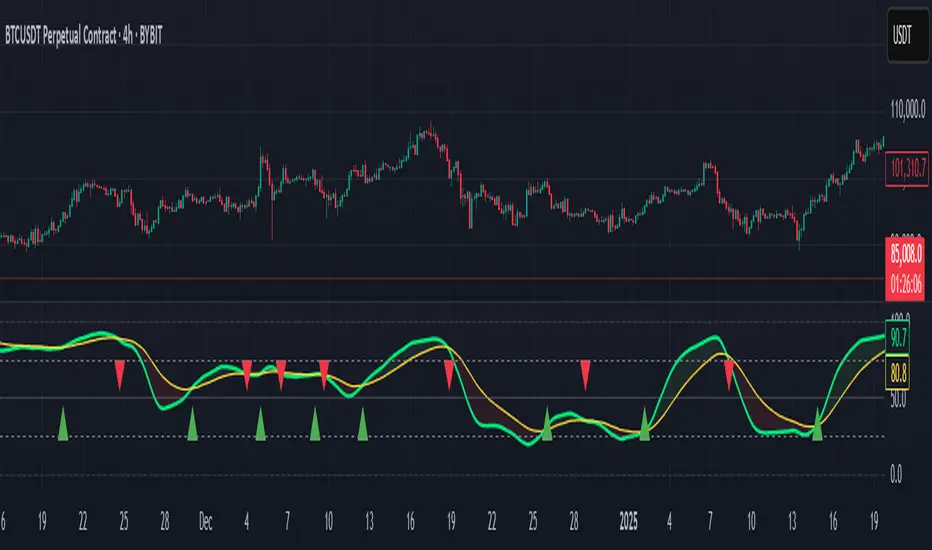
Kase Permission StochasticOverview
The Kase Permission Stochastic indicator is an advanced momentum oscillator developed from Kase's trading methodology. It offers enhanced signal smoothing and filtering compared to traditional stochastic oscillators, providing clearer entry and exit signals with fewer false triggers.
How It Works
This indicator calculates a specialized stochastic using a multi-stage smoothing process:
Initial stochastic calculation based on high, low, and close prices
Application of weighted moving averages (WMA) for short-term smoothing
Progressive smoothing through differential factors
Final smoothing to reduce noise and highlight significant trend changes
The indicator oscillates between 0 and 100, with two main components:
Main Line (Green): The smoothed stochastic value
Signal Line (Yellow): A further smoothed version of the main line
Signal Generation
Trading signals are generated when the main line crosses the signal line:
Buy Signal (Green Triangle): When the main line crosses above the signal line
Sell Signal (Red Triangle): When the main line crosses below the signal line
Key Features
Multiple Smoothing Algorithms: Uses a combination of weighted and exponential moving averages for superior noise reduction
Clear Visualization: Color-coded lines and background filling
Reference Levels: Horizontal lines at 25, 50, and 75 for context
Customizable Colors: All visual elements can be color-customized
Customization Options
PST Length: Base period for the stochastic calculation (default: 9)
PST X: Multiplier for the lookback period (default: 5)
PST Smooth: Smoothing factor for progressive calculations (default: 3)
Smooth Period: Final smoothing period (default: 10)
Trading Applications
Trend Confirmation: Use crossovers to confirm entries in the direction of the prevailing trend
Reversal Detection: Identify potential market reversals when crossovers occur at extreme levels
Range-Bound Markets: Look for oscillations between overbought and oversold levels
Filter for Other Indicators: Use as a confirmation tool alongside other technical indicators
Best Practices
Most effective in trending markets or during well-defined ranges
Combine with price action analysis for better context
Consider the overall market environment before taking signals
Use longer settings for fewer but higher-quality signals
The Kase Permission Stochastic delivers a sophisticated approach to momentum analysis, offering a refined perspective on market conditions while filtering out much of the noise that affects standard oscillators.
Buscar en scripts para "algo"
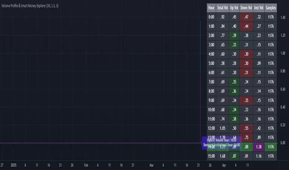
Volume Profile & Smart Money Explorer🔍 Volume Profile & Smart Money Explorer: Decode Institutional Footprints
Master the art of institutional trading with this sophisticated volume analysis tool. Track smart money movements, identify peak liquidity windows, and align your trades with major market participants.
🌟 Key Features:
📊 Triple-Layer Volume Analysis
• Total Volume Patterns
• Directional Volume Split (Up/Down)
• Institutional Flow Detection
• Real-time Smart Money Tracking
• Historical Pattern Recognition
⚡ Smart Money Detection
• Institutional Trade Identification
• Large Block Order Tracking
• Smart Money Concentration Periods
• Whale Activity Alerts
• Volume Threshold Analysis
📈 Advanced Profiling
• Hourly Volume Distribution
• Directional Bias Analysis
• Liquidity Heat Maps
• Volume Pattern Recognition
• Custom Threshold Settings
🎯 Strategic Applications:
Institutional Trading:
• Track Big Player Movements
• Identify Accumulation/Distribution
• Follow Smart Money Flow
• Detect Institutional Trading Windows
• Monitor Block Orders
Risk Management:
• Identify High Liquidity Windows
• Avoid Thin Market Periods
• Optimize Position Sizing
• Track Market Participation
• Monitor Volume Quality
Market Analysis:
• Volume Pattern Recognition
• Smart Money Flow Analysis
• Liquidity Window Identification
• Institutional Activity Cycles
• Market Depth Analysis
💡 Perfect For:
• Professional Traders
• Volume Profile Traders
• Institutional Traders
• Risk Managers
• Algorithmic Traders
• Smart Money Followers
• Day Traders
• Swing Traders
📊 Key Metrics:
• Normalized Volume Profiles
• Institutional Thresholds
• Directional Volume Split
• Smart Money Concentration
• Historical Patterns
• Real-time Analysis
⚡ Trading Edge:
• Trade with Institution Flow
• Identify Optimal Entry Points
• Recognize Distribution Patterns
• Follow Smart Money Positioning
• Avoid Thin Markets
• Capitalize on Peak Liquidity
🎓 Educational Value:
• Understand Market Structure
• Learn Volume Analysis
• Master Institutional Patterns
• Develop Market Intuition
• Track Smart Money Flow
🛠️ Customization:
• Adjustable Time Windows
• Flexible Volume Thresholds
• Multiple Timeframe Analysis
• Custom Alert Settings
• Visual Preference Options
Whether you're tracking institutional flows in crypto markets or following smart money in traditional markets, the Volume Profile & Smart Money Explorer provides the deep insights needed to trade alongside the biggest players.
Transform your trading from retail guesswork to institutional precision. Know exactly when and where smart money moves, and position yourself ahead of major market shifts.
#VolumeProfile #SmartMoney #InstitutionalTrading #MarketAnalysis #TradingView #VolumeAnalysis #CryptoTrading #ForexTrading #TechnicalAnalysis #Trading #PriceAction #MarketStructure #OrderFlow #Liquidity #RiskManagement #TradingStrategy #DayTrading #SwingTrading #AlgoTrading #QuantitativeTrading
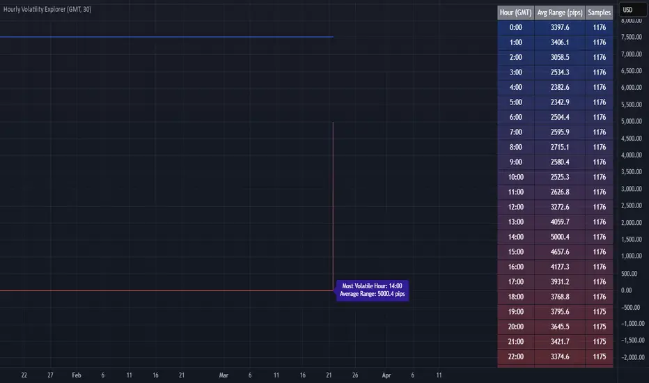
Hourly Volatility Explorer📊 Hourly Volatility Explorer: Master The Market's Pulse
Unlock the hidden rhythms of price action with this sophisticated volatility analysis tool. The Hourly Volatility Explorer reveals the most potent trading hours across multiple time zones, giving you a strategic edge in timing your trades.
🌟 Key Features:
⏰ Multi-Timezone Analysis
• GMT (UTC+0)
• EST (UTC-5) - New York
• BST (UTC+1) - London
• JST (UTC+9) - Tokyo
• AEST (UTC+10) - Sydney
Perfect for tracking major market sessions and their overlaps!
📈 Dynamic Visualization
• Color-gradient hourly bars for instant pattern recognition
• Real-time volatility comparison
• Interactive data table with comprehensive statistics
• Automatic highlighting of peak volatility periods
🎯 Strategic Applications:
Day Trading:
• Identify optimal trading windows
• Avoid low-liquidity periods
• Capitalize on session overlaps
• Fine-tune entry/exit timing
Risk Management:
• Set appropriate stop losses based on hourly volatility
• Adjust position sizes for different market hours
• Optimize risk-reward ratios
• Plan around high-impact hours
Global Market Analysis:
• Track volatility across all major sessions
• Spot institutional trading patterns
• Identify quiet vs. active periods
• Monitor 24/7 market dynamics
💡 Perfect For:
• Forex traders navigating global sessions
• Crypto traders in 24/7 markets
• Day traders optimizing execution times
• Algorithmic traders fine-tuning strategies
• Risk managers calibrating exposure
📊 Advanced Features:
• Rolling 3-month analysis for reliable patterns
• Precise pip movement calculations
• Sample size tracking for statistical validity
• Real-time current hour comparison
• Color-coded visual system for instant insights
⚡ Pro Trading Tips:
• Use during major session overlaps for maximum opportunity
• Compare patterns across different instruments
• Combine with volume analysis for deeper insights
• Track seasonal variations in hourly patterns
• Build trading schedules around peak hours
🎓 Educational Value:
• Understand market microstructure
• Learn global market dynamics
• Master timezone relationships
• Develop timing intuition
🛠️ Customization:
• Adjustable lookback period
• Flexible pip multiplier
• Multiple timezone options
• Visual preference settings
Whether you're scalping the 1-minute chart or managing longer-term positions, the Hourly Volatility Explorer provides the precise timing intelligence needed for today's global markets.
Transform your trading schedule from guesswork to science. Know exactly when markets move, why they move, and how to position yourself for maximum opportunity.
#TechnicalAnalysis #Trading #Volatility #MarketTiming #DayTrading #Forex #Crypto #TradingView #PineScript #MarketAnalysis #TradingStrategy #RiskManagement #GlobalMarkets #FinancialMarkets #TradingTools #MarketStructure #PriceAction #Scalping #SwingTrading #AlgoTrading
VIDYA For-Loop | QuantEdgeB Introducing VIDYA For-Loop by QuantEdgeB
Overview
The VIDYA For-Loop indicator by QuantEdgeB is a dynamic trend-following tool that leverages Variable Index Dynamic Average (VIDYA) along with a rolling loop function to assess trend strength and direction. By utilizing adaptive smoothing and a recursive loop for threshold evaluation, this indicator provides a more responsive and robust signal framework for traders.
______
Key Components & Features
📌 VIDYA (Variable Index Dynamic Average)
- Adaptive Moving Average that adjusts its responsiveness based on market volatility.
- Uses a dynamic smoothing constant based on standard deviations.
- Allows for better trend detection compared to static moving averages.
📌 Loop Function (Rolling Calculation)
- A for-loop algorithm continuously compares VIDYA values over a defined lookback range.
- Measures the number of times price trends higher or lower within the rolling window.
- Generates a momentum-based score that helps quantify trend persistence.
📌 Trend Signal Calculation
- A long signal is triggered when the loop score exceeds the upper threshold.
- A short signal is triggered when the loop score falls below the lower threshold.
- The result is a clear directional bias that adapts to changing market conditions.
______
How It Works in Trading
✅ Detects Trend Strength – By measuring cumulative movements within a window.
✅ Filters Noise – Uses adaptive smoothing to avoid whipsaws.
✅ Dynamic Thresholds – Enables customized entry & exit conditions.
✅ Color-Coded Candles – Provides visual clarity for traders.
______
Visual Representation
Trend Signals:
🔵 Blue Candles – Strong Uptrend
🔴 Red Candles – Strong Downtrend
Thresholds:
📈 Long Threshold – Upper bound for bullish confirmation.
📉 Short Threshold – Lower bound for bearish confirmation.
Labels & Annotations (Optional):
✅ Long & Short Labels can be turned on or off for trade signal clarity.
📊 Display of entry & exit points based on loop calculations.
______
Settings:
VIDYA Length: 2 → Number of bars for VIDYA calculation.
SD Length: 5 → Standard deviation length for VIDYA calculation.
Source: Close → Defines the input data source (Close price).
Start Loop: 1 → Initial lookback period for the loop function.
End Loop: 60 → Maximum lookback range for trend scoring.
Long Threshold: 40 → Upper bound for a long signal.
Short Threshold: 10 → Lower bound for a short signal.
Extra Plots: True → Enables additional moving averages for visualization.
______
Conclusion
The VIDYA For-Loop by QuantEdgeB is a next-gen adaptive trend filter that combines dynamic smoothing with recursive trend evaluation, making it an invaluable tool for traders seeking precision and consistency in their strategies.
🔹 Who should use VIDYA For Loop :
📊 Trend-Following Traders – Helps identify sustained trends.
⚡ Momentum Traders – Captures strong price swings.
🚀 Algorithmic & Systematic Trading – Ideal for automated entries & exits.
🔹 Disclaimer: Past performance is not indicative of future results. No trading strategy can guarantee success in financial markets.
🔹 Strategic Advice: Always backtest, optimize, and align parameters with your trading objectives and risk tolerance before live trading.

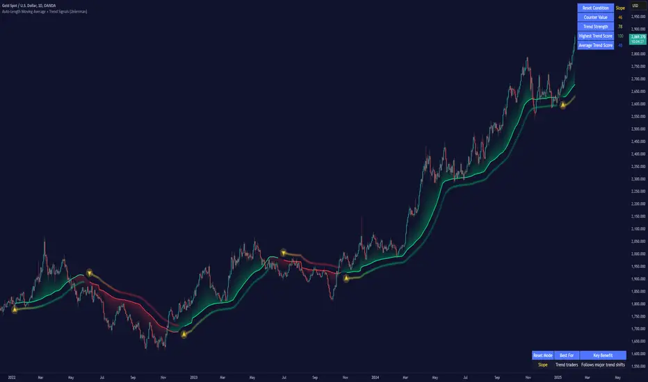
Auto-Length Moving Average + Trend Signals (Zeiierman)█ Overview
The Auto-Length Moving Average + Trend Signals (Zeiierman) is an easy-to-use indicator designed to help traders dynamically adjust their moving average length based on market conditions. This tool adapts in real-time, expanding and contracting the moving average based on trend strength and momentum shifts.
The indicator smooths out price fluctuations by modifying its length while ensuring responsiveness to new trends. In addition to its adaptive length algorithm, it incorporates trend confirmation signals, helping traders identify potential trend reversals and continuations with greater confidence.
This indicator suits scalpers, swing traders, and trend-following investors who want a self-adjusting moving average that adapts to volatility, momentum, and price action dynamics.
█ How It Works
⚪ Dynamic Moving Average Length
The core feature of this indicator is its ability to automatically adjust the length of the moving average based on trend persistence and market conditions:
Expands in strong trends to reduce noise.
Contracts in choppy or reversing markets for faster reaction.
This allows for a more accurate moving average that aligns with current price dynamics.
⚪ Trend Confirmation & Signals
The indicator includes built-in trend detection logic, classifying trends based on market structure. It evaluates trend strength based on consecutive bars and smooths out transitions between bullish, bearish, and neutral conditions.
Uptrend: Price is persistently above the adjusted moving average.
Downtrend: Price remains below the adjusted moving average.
Neutral: Price fluctuates around the moving average, indicating possible consolidation.
⚪ Adaptive Trend Smoothing
A smoothing factor is applied to enhance trend readability while minimizing excessive lag. This balances reactivity with stability, making it easier to follow longer-term trends while avoiding false signals.
█ How to Use
⚪ Trend Identification
Bullish Trend: The indicator confirms an uptrend when the price consistently stays above the dynamically adjusted moving average.
Bearish Trend: A downtrend is recognized when the price remains below the moving average.
⚪ Trade Entry & Exit
Enter long when the dynamic moving average is green and a trend signal occurs. Exit when the price crosses below the dynamic moving average.
Enter short when the dynamic moving average is red and a trend signal occurs. Exit when the price crosses above the dynamic moving average.
█ Slope-Based Reset
This mode resets the trend counter when the moving average slope changes direction.
⚪ Interpretation & Insights
Best for trend-following traders who want to filter out noise and only reset when a clear shift in momentum occurs.
Higher slope length (N): More stable trends, fewer resets.
Lower slope length (N): More reactive to small price swings, frequent resets.
Useful in swing trading to track significant trend reversals.
█ RSI-Based Reset
The counter resets when the Relative Strength Index (RSI) crosses predefined overbought or oversold levels.
⚪ Interpretation & Insights
Best for reversal traders who look for extreme overbought/oversold conditions.
High RSI threshold (e.g., 80/20): Fewer resets, only extreme conditions trigger adjustments.
Lower RSI threshold (e.g., 60/40): More frequent resets, detecting smaller corrections.
Great for detecting exhaustion in trends before potential reversals.
█ Volume-Based Reset
A reset occurs when current volume significantly exceeds its moving average, signaling a shift in market participation.
⚪ Interpretation & Insights
Best for traders who follow institutional activity (high volume often means large players are active).
Higher volume SMA length: More stable trends, only resets on massive volume spikes.
Lower volume SMA length: More reactive to short-term volume shifts.
Useful in identifying breakout conditions and trend acceleration points.
█ Bollinger Band-Based Reset
A reset occurs when price closes above the upper Bollinger Band or below the lower Bollinger Band, signaling potential overextension.
⚪ Interpretation & Insights
Best for traders looking for volatility-based trend shifts.
Higher Bollinger Band multiplier (k = 2.5+): Captures only major price extremes.
Lower Bollinger Band multiplier (k = 1.5): Resets on moderate volatility changes.
Useful for detecting overextensions in strong trends before potential retracements.
█ MACD-Based Reset
A reset occurs when the MACD line crosses the signal line, indicating a momentum shift.
⚪ Interpretation & Insights
Best for momentum traders looking for trend continuation vs. exhaustion signals.
Longer MACD lengths (260, 120, 90): Captures major trend shifts.
Shorter MACD lengths (10, 5, 3): Reacts quickly to momentum changes.
Useful for detecting strong divergences and market shifts.
█ Stochastic-Based Reset
A reset occurs when Stochastic %K crosses overbought or oversold levels.
⚪ Interpretation & Insights
Best for short-term traders looking for fast momentum shifts.
Longer Stochastic length: Filters out false signals.
Shorter Stochastic length: Captures quick intraday shifts.
█ CCI-Based Reset
A reset occurs when the Commodity Channel Index (CCI) crosses predefined overbought or oversold levels. The CCI measures the price deviation from its statistical mean, making it a useful tool for detecting overextensions in price action.
⚪ Interpretation & Insights
Best for cycle traders who aim to identify overextended price deviations in trending or ranging markets.
Higher CCI threshold (e.g., ±200): Detects extreme overbought/oversold conditions before reversals.
Lower CCI threshold (e.g., ±10): More sensitive to trend shifts, useful for early signal detection.
Ideal for detecting momentum shifts before price reverts to its mean or continues trending strongly.
█ Momentum-Based Reset
A reset occurs when Momentum (Rate of Change) crosses zero, indicating a potential shift in price direction.
⚪ Interpretation & Insights
Best for trend-following traders who want to track acceleration vs. deceleration.
Higher momentum length: Captures longer-term shifts.
Lower momentum length: More responsive to short-term trend changes.
█ How to Interpret the Trend Strength Table
The Trend Strength Table provides valuable insights into the current market conditions by tracking how the dynamic moving average is adjusting based on trend persistence. Each metric in the table plays a role in understanding the strength, longevity, and stability of a trend.
⚪ Counter Value
Represents the current length of trend persistence before a reset occurs.
The higher the counter, the longer the current trend has been in place without resetting.
When this value reaches the Counter Break Threshold, the moving average resets and contracts to become more reactive.
Example:
A low counter value (e.g., 10) suggests a recent trend reset, meaning the market might be changing directions frequently.
A high counter value (e.g., 495) means the trend has been ongoing for a long time, indicating strong trend persistence.
⚪ Trend Strength
Measures how strong the current trend is based on the trend confirmation logic.
Higher values indicate stronger trends, while lower values suggest weaker trends or consolidations.
This value is dynamic and updates based on price action.
Example:
Trend Strength of 760 → Indicates a high-confidence trend.
Trend Strength of 50 → Suggests weak price action, possibly a choppy market.
⚪ Highest Trend Score
Tracks the strongest trend score recorded during the session.
Helps traders identify the most dominant trend observed in the timeframe.
This metric is useful for analyzing historical trend strength and comparing it with current conditions.
Example:
Highest Trend Score = 760 → Suggests that at some point, there was a strong trend in play.
If the current trend strength is much lower than this value, it could indicate trend exhaustion.
⚪ Average Trend Score
This is a rolling average of trend strength across the session.
Provides a bigger picture of how the trend strength fluctuates over time.
If the average trend score is high, the market has had persistent trends.
If it's low, the market may have been choppy or sideways.
Example:
Average Trend Score of 147 vs. Current Trend Strength of 760 → Indicates that the current trend is significantly stronger than the historical average, meaning a breakout might be occurring.
Average Trend Score of 700+ → Suggests a strong trending market overall.
█ Settings
⚪ Dynamic MA Controls
Base MA Length – Sets the starting length of the moving average before dynamic adjustments.
Max Dynamic Length – Defines the upper limit for how much the moving average can expand.
Trend Confirmation Length – The number of bars required to validate an uptrend or downtrend.
⚪ Reset & Adaptive Conditions
Reset Condition Type – Choose what triggers the moving average reset (Slope, RSI, Volume, MACD, etc.).
Trend Smoothing Factor – Adjusts how smoothly the moving average responds to price changes.
-----------------
Disclaimer
The content provided in my scripts, indicators, ideas, algorithms, and systems is for educational and informational purposes only. It does not constitute financial advice, investment recommendations, or a solicitation to buy or sell any financial instruments. I will not accept liability for any loss or damage, including without limitation any loss of profit, which may arise directly or indirectly from the use of or reliance on such information.
All investments involve risk, and the past performance of a security, industry, sector, market, financial product, trading strategy, backtest, or individual's trading does not guarantee future results or returns. Investors are fully responsible for any investment decisions they make. Such decisions should be based solely on an evaluation of their financial circumstances, investment objectives, risk tolerance, and liquidity needs.
2022 Model ICT Entry Strategy [TradingFinder] One Setup For Life🔵 Introduction
The ICT 2022 model, introduced by Michael Huddleston, is an advanced trading strategy rooted in liquidity and price imbalance, where time and price serve as the core elements. This ICT 2022 trading strategy is an algorithmic approach designed to analyze liquidity and imbalances in the market. It incorporates concepts such as Fair Value Gap (FVG), Liquidity Sweep, and Market Structure Shift (MSS) to help traders identify liquidity movements and structural changes in the market, enabling them to determine optimal entry and exit points for their trades.
This Full ICT Day Trading Model empowers traders to pinpoint the Previous Day High/Low as well as the highs and lows of critical sessions like the London and New York sessions. These levels act as Liquidity Zones, which are frequently swept prior to a market structure shift (MSS) or a retracement to areas such as Optimal Trade Entry (OTE).
Bullish :
Bearish :
🔵 How to Use
The ICT 2022 model is a sophisticated trading strategy that focuses on identifying key liquidity levels and price movements. It operates based on two main principles. In the first phase, the price approaches liquidity zones and sweeps critical levels such as the previous day’s high or low and key session levels.
This movement is known as a Liquidity Sweep. In the second phase, following the sweep, the price retraces to areas like the FVG (Fair Value Gap), creating ideal entry points for trades. Below is a detailed explanation of how to apply this strategy in bullish and bearish setups.
🟣 Bullish ICT 2022 Model Setup
To use the ICT 2022 model in a bullish setup, start by identifying the Previous Day High/Low or key session levels, such as those of the London or New York sessions. In a bullish setup, the price usually moves downward first, sweeping the Liquidity Low. This move, known as a Liquidity Sweep, reflects the collection of buy orders by major market participants.
After the liquidity sweep, the price should shift market structure and start moving upward; this shift, referred to as Market Structure Shift (MSS), signals the beginning of an upward trend. Following MSS, areas like FVG, located within the Discount Zone, are identified. At this stage, the trader waits for the price to retrace to these zones. Once the price returns, a long trade is executed.
Finally, the stop-loss should be set below the liquidity low to manage risk, while the take-profit target is usually placed above the previous day’s high or other identified liquidity levels. This structure enables traders to take advantage of the upward price movement after the liquidity sweep.
🟣 Bearish ICT 2022 Model Setup
To identify a bearish setup in the ICT 2022 model, begin by marking the Previous Day High/Low or key session levels, such as the London or New York sessions. In this scenario, the price typically moves upward first, sweeping the Liquidity High. This move, known as a Liquidity Sweep, signifies the collection of sell orders by key market players.
After the liquidity sweep, the price should shift market structure downward. This movement, called the Market Structure Shift (MSS), indicates the start of a downtrend. Following MSS, areas such as FVG, found within the Premium Zone, are identified. At this stage, the trader waits for the price to retrace to these areas. Once the price revisits these zones, a short trade is executed.
In this setup, the stop-loss should be placed above the liquidity high to control risk, while the take-profit target is typically set below the previous day’s low or another defined liquidity level. This approach allows traders to capitalize on the downward price movement following the liquidity sweep.
🔵 Settings
Swing period : You can set the swing detection period.
Max Swing Back Method : It is in two modes "All" and "Custom". If it is in "All" mode, it will check all swings, and if it is in "Custom" mode, it will check the swings to the extent you determine.
Max Swing Back : You can set the number of swings that will go back for checking.
FVG Length : Default is 120 Bar.
MSS Length : Default is 80 Bar.
FVG Filter : This refines the number of identified FVG areas based on a specified algorithm to focus on higher quality signals and reduce noise.
Types of FVG filters :
Very Aggressive Filter: Adds a condition where, for an upward FVG, the last candle's highest price must exceed the middle candle's highest price, and for a downward FVG, the last candle's lowest price must be lower than the middle candle's lowest price. This minimally filters out FVGs.
Aggressive Filter: Builds on the Very Aggressive mode by ensuring the middle candle is not too small, filtering out more FVGs.
Defensive Filter: Adds criteria regarding the size and structure of the middle candle, requiring it to have a substantial body and specific polarity conditions, filtering out a significant number of FVGs.
Very Defensive Filter: Further refines filtering by ensuring the first and third candles are not small-bodied doji candles, retaining only the highest quality signals.
🔵 Conclusion
The ICT 2022 model is a comprehensive and advanced trading strategy designed around key concepts such as liquidity, price imbalance, and market structure shifts (MSS). By focusing on the sweep of critical levels such as the previous day’s high/low and important trading sessions like London and New York, this strategy enables traders to predict market movements with greater precision.
The use of tools like FVG in this model helps traders fine-tune their entry and exit points and take advantage of bullish and bearish trends after liquidity sweeps. Moreover, combining this strategy with precise timing during key trading sessions allows traders to minimize risk and maximize returns.
In conclusion, the ICT 2022 model emphasizes the importance of time and liquidity, making it a powerful tool for both professional and novice traders. By applying the principles of this model, you can make more informed trading decisions and seize opportunities in financial markets more effectively.

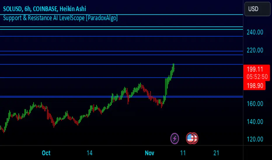
Support & Resistance AI LevelScopeSupport & Resistance AI LevelScope
Support & Resistance AI LevelScope is an advanced, AI-driven tool that automatically detects and highlights key support and resistance levels on your chart. This indicator leverages smart algorithms to pinpoint the most impactful levels, providing traders with a precise, real-time view of critical price boundaries. Save time and enhance your trading edge with effortless, intelligent support and resistance identification.
Key Features:
AI-Powered Level Detection: The LevelScope algorithm continuously analyzes price action, dynamically plotting support and resistance levels based on recent highs and lows across your chosen timeframe.
Sensitivity Control: Customize the sensitivity to display either major levels for a macro view or more frequent levels for detailed intraday analysis. Easily adjust to suit any trading style or market condition.
Level Strength Differentiation: Instantly recognize the strength of each level with visual cues based on how often price has touched each one. Stronger levels are emphasized, highlighting areas with higher significance, while weaker levels are marked subtly.
Customizable Visuals: Tailor the look of your chart with customizable color schemes and line thickness options for strong and weak levels, ensuring clear visibility without clutter.
Proximity Alerts: Receive alerts when price approaches key support or resistance, giving you a heads-up for potential market reactions and trading opportunities.
Who It’s For:
Whether you're a day trader, swing trader, or just want a quick, AI-driven way to identify high-probability levels on your chart, Support & Resistance AI LevelScope is designed to keep you focused and informed. This indicator is the perfect addition to any trader’s toolkit, empowering you to make more confident, data-backed trading decisions with ease.
Upgrade your analysis with AI-powered support and resistance—no more manual lines, only smart levels!
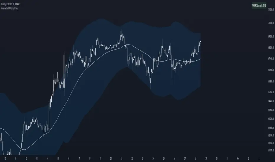
Advanced VWAP [CryptoSea]The Advanced VWAP is a comprehensive volume-weighted average price (VWAP) tool designed to provide traders with a deeper understanding of market trends through multi-layered VWAP analysis. This indicator is ideal for those who want to track price movements in relation to VWAP bands and detect key market levels with greater precision.
Key Features
Multi-Timeframe VWAP Bands: Includes multiple VWAP bands with different lookback periods (5, 10, 25, and 50), allowing traders to observe short-term and long-term price behavior.
Smoothed Band Options: Offers optional smoothing of VWAP bands to reduce noise and highlight significant trends more clearly.
Dynamic Median Line Display: Plots the median line of the VWAP bands, providing a reference for price movements and potential reversal zones.
VWAP Trend Strength Calculation: Measures the strength of the trend based on the price's position relative to the VWAP bands, normalized between -1 and 1 for easier interpretation.
In the example below we can see the VWAP Forecastd Cloud, which consists of multiple layers of VWAP bands with varying lookback periods, creating a dynamic forecast visualization. The cloud structure represents potential future price ranges by projecting VWAP-based bands outward, with darker areas indicating higher density and overlap of the bands, suggesting stronger support or resistance zones. This approach helps traders anticipate price movement and identify areas of potential consolidation or breakout as the price interacts with different layers of the forecast cloud.
How it Works
VWAP Calculation: Utilizes multiple VWAP calculations based on various lookback periods to capture a broad range of price behaviors. The indicator adapts to different market conditions by switching between short-term and long-term VWAP references.
Smoothing Algorithms: Provides the ability to smooth the VWAP bands using different moving average types (SMA, EMA, SMMA, WMA, VWMA) to suit various trading strategies and reduce market noise.
Trend Strength Analysis: Computes the trend strength based on the price's distance from the VWAP bands, with a value range of -1 to 1. This feature helps traders identify the intensity of uptrends and downtrends.
Alert Conditions: Includes alert options for crossing above or below the smoothed median line, as well as touching the smoothed upper or lower bands, providing timely notifications for potential trading opportunities.
This image below illustrates the use of smoothed VWAP bands, which provide a cleaner representation of the price's relationship to the VWAP by reducing market noise. The smoothed bands create a flowing cloud-like structure, making it easier to observe significant trends and potential reversal points. The circles highlight areas where the price interacts with the smoothed bands, indicating potential key levels for trend continuation or reversal. This setup helps traders focus on meaningful movements and filter out minor fluctuations, improving the identification of strategic entry and exit points based on smoother trend signals.
Application
Strategic Entry and Exit Points: Helps traders identify optimal entry and exit points based on the interaction with VWAP bands and trend strength readings.
Trend Confirmation: Assists in confirming trend strength by analyzing price movements relative to the VWAP bands and detecting significant breaks or touches.
Customized Analysis: Supports a wide range of trading styles by offering adjustable smoothing, band settings, and alert conditions to meet specific trading needs.
The Advanced VWAP by is a valuable addition to any trader's toolkit, offering versatile features to navigate different market scenarios with confidence. Whether used for day trading or longer-term analysis, this tool enhances decision-making by providing a robust view of price behavior relative to VWAP levels.
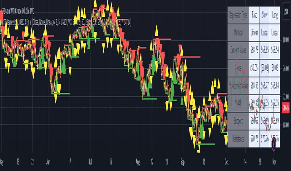
MTF Regression with Forecast### **MTF Regression with Forecast, Treasury Yield, Additional Variable & VWAP Filter - Enhanced with Long Regression**
Unlock advanced market insights with our **MTF Regression** indicator, meticulously designed for traders seeking comprehensive multi-timeframe analysis combined with powerful forecasting tools. Whether you're a seasoned trader or just starting out, this indicator offers a suite of features to enhance your trading strategy.
#### **🔍 Key Features:**
- **Multi-Timeframe (MTF) Regression:**
- **Fast, Slow, & Long Regressions:** Analyze price trends across multiple timeframes to capture both short-term movements and long-term trends.
- **Customizable Price Inputs:**
- **Flexible Price Selection:** Choose between Close, Open, High, or Low prices to suit your trading style.
- **Price Transformation:** Option to apply Exponential Moving Averages (EMA) for smoother trend analysis.
- **Diverse Regression Methods:**
- **Multiple Algorithms:** Select from Linear, Exponential, Hull Moving Average (HMA), Weighted Moving Average (WMA), or Spline regressions to best fit your analysis needs.
- **Integrated External Data:**
- **10-Year Treasury Yield:** Incorporate macroeconomic indicators to refine regression accuracy.
- **Additional Variables:** Enhance your analysis by integrating data from other tickers (e.g., NASDAQ:AAPL).
- **Advanced Filtering Options:**
- **VWAP Filter:** Align signals with the Volume Weighted Average Price for improved trade entries.
- **Price Action Filter:** Ensure price behavior supports the generated signals for higher reliability.
- **Enhanced Signal Generation:**
- **Bullish & Bearish Signals:** Identify potential trend reversals and continuations with clear visual cues.
- **Predictive Signals:** Forecast future price movements with forward-looking arrows based on regression slopes.
- **Slope & Acceleration Thresholds:** Customize minimum slope and acceleration levels to fine-tune signal sensitivity.
- **Forecasting Capabilities:**
- **Projection Lines:** Visualize future price trends by extending regression lines based on current slope data.
- **User-Friendly Interface:**
- **Organized Settings Groups:** Easily navigate through price inputs, regression settings, integration options, and more.
- **Customizable Alerts:** Stay informed with configurable alerts for bullish, bearish, and predictive signals.
#### **📈 Why Choose MTF Regression Indicator?**
- **Comprehensive Analysis:** Combines multiple regression techniques and external data sources for a well-rounded market view.
- **Flexibility:** Highly customizable to fit various trading strategies and preferences.
- **Enhanced Decision-Making:** Provides clear signals and forecasts to support informed trading decisions.
- **Efficiency:** Optimized to deliver reliable performance without overloading your trading platform.
Elevate your trading game with the **MTF Regression with Forecast, Treasury Yield, Additional Variable & VWAP Filter** indicator. Harness the power of multi-timeframe analysis and predictive forecasting to stay ahead in the dynamic markets.
---
*Feel free to reach out for more information or support. Happy Trading!*
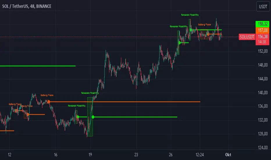
Iceberg Trade Revealer [CHE]Unveiling Iceberg Trades: A Deep Dive into Low Volatility Market Phases
Introduction
In the dynamic world of trading, hidden forces often influence market movements in ways that aren't immediately apparent. One such force is the phenomenon of iceberg trades—large orders that are concealed to prevent significant market impact. This presentation explores the concept of iceberg trades, explains why they are typically hidden during periods of low volatility, and introduces an indicator designed to reveal these elusive trades.
Agenda
1. Understanding Iceberg Trades
- Definition and Purpose
- Impact on Market Dynamics
2. The Low Volatility Concealment
- Why Low Volatility Phases?
- Strategies Behind Hiding Large Orders
3. Introducing the Iceberg Trade Revealer Indicator
- How the Indicator Works
- Key Components and Calculations
4. Demonstration and Use Cases
- Interpreting the Indicator Signals
- Practical Trading Applications
5. Conclusion
- Summarizing the Insights
- Q&A Session
1. Understanding Iceberg Trades
Definition and Purpose
- Iceberg Trades are large single orders divided into smaller lots to disguise the total order quantity.
- Traders use iceberg orders to minimize market impact and avoid unfavorable price movements.
Impact on Market Dynamics
- Concealed Volume: Iceberg orders hide true supply and demand levels.
- Price Stability: They prevent sudden spikes or drops by releasing orders gradually.
- Market Sentiment: Their presence can influence perceptions of market strength or weakness.
2. The Low Volatility Concealment
Why Low Volatility Phases?
- Less Market Attention: Low volatility periods attract fewer traders, making it easier to conceal large orders.
- Reduced Slippage: Prices are more stable, reducing the risk of executing orders at unfavorable prices.
- Strategic Advantage: Large players can accumulate or distribute positions without tipping off the market.
Strategies Behind Hiding Large Orders
- Order Splitting: Breaking down large orders into smaller pieces.
- Time Slicing: Executing orders over an extended period.
- Algorithmic Trading: Using sophisticated algorithms to optimize order execution.
3. Introducing the Iceberg Trade Revealer Indicator
How the Indicator Works
- Core Thesis: Iceberg trades can be detected by analyzing periods of unusually low volatility.
- Volatility Analysis: Uses the Average True Range (ATR) and Bollinger Bands to identify low volatility phases.
- Signal Generation: Marks periods where iceberg trades are likely occurring.
Key Components and Calculations
1. Average True Range (ATR)
- Measures market volatility over a specified period.
- Lower ATR values indicate less price movement.
2. Bollinger Bands
- Creates a volatility envelope around the ATR.
- Bands tighten during low volatility and widen during high volatility.
3. Timeframe Adjustments
- Utilizes multiple timeframes to enhance signal accuracy.
- Options for auto, multiplier, or manual timeframe selection.
4. Signal Conditions
- Iceberg Trade Detection: ATR falls below the lower Bollinger Band.
- Revealed Volatility: ATR rises above the upper Bollinger Band, indicating potential market moves after iceberg trades.
4. Demonstration and Use Cases
Interpreting the Indicator Signals
- Iceberg Trade Zones: Highlighted areas where large hidden orders are likely.
- Revealed Volatility Zones: Areas indicating the market's response to the execution of iceberg trades.
Practical Trading Applications
- Entry and Exit Points: Use signals to time trades alongside institutional activity.
- Risk Management: Adjust strategies during detected low volatility phases.
- Market Analysis: Gain insights into underlying market mechanics.
5. Conclusion
Summarizing the Insights
- Iceberg Trades play a significant role in market movements, especially when concealed during low volatility phases.
- The Iceberg Trade Revealer Indicator provides a tool to uncover these hidden activities, offering traders a strategic edge.
- Understanding and utilizing this indicator can enhance trading decisions by aligning them with the actions of major market players.
Best regards Chervolino ( Volker )
Q&A Session
- Questions and Discussions: Open the floor for any queries or further explanations.
Thank You!
By delving into the hidden aspects of market activity, traders can better navigate the complexities of financial markets. The Iceberg Trade Revealer Indicator serves as a bridge between observable market data and the concealed strategies of large institutions.
References
- Average True Range (ATR): A technical analysis indicator that measures market volatility.
- Bollinger Bands: A volatility indicator that creates a band of three lines which are plotted in relation to a security's price.
- Iceberg Orders: Large orders divided into smaller lots to hide the actual order quantity.
Note: Always consider multiple factors when making trading decisions. Indicators provide tools, but they do not guarantee results.
Educational Content Disclaimer:
Disclaimer:
The content provided, including all code and materials, is strictly for educational and informational purposes only. It is not intended as, and should not be interpreted as, financial advice, a recommendation to buy or sell any financial instrument, or an offer of any financial product or service. All strategies, tools, and examples discussed are provided for illustrative purposes to demonstrate coding techniques and the functionality of Pine Script within a trading context.
Any results from strategies or tools provided are hypothetical, and past performance is not indicative of future results. Trading and investing involve high risk, including the potential loss of principal, and may not be suitable for all individuals. Before making any trading decisions, please consult with a qualified financial professional to understand the risks involved.
By using this script, you acknowledge and agree that any trading decisions are made solely at your discretion and risk.
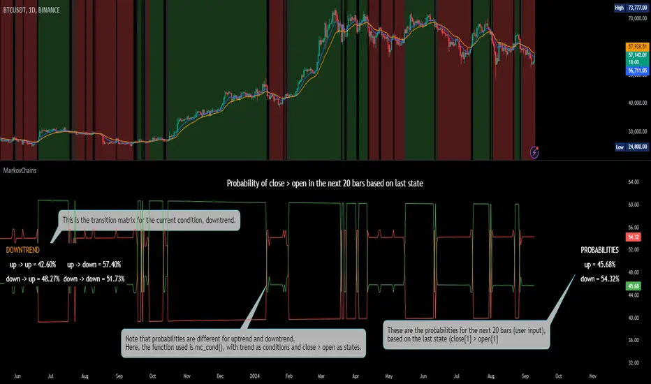
[ALGOA+] Markov Chains Library by @metacamaleoLibrary "MarkovChains"
Markov Chains library by @metacamaleo. Created in 09/08/2024.
This library provides tools to calculate and visualize Markov Chain-based transition matrices and probabilities. This library supports two primary algorithms: a rolling window Markov Chain and a conditional Markov Chain (which operates based on specified conditions). The key concepts used include Markov Chain states, transition matrices, and future state probabilities based on past market conditions or indicators.
Key functions:
- `mc_rw()`: Builds a transition matrix using a rolling window Markov Chain, calculating probabilities based on a fixed length of historical data.
- `mc_cond()`: Builds a conditional Markov Chain transition matrix, calculating probabilities based on the current market condition or indicator state.
Basically, you will just need to use the above functions on your script to default outputs and displays.
Exported UDTs include:
- s_map: An UDT variable used to store a map with dummy states, i.e., if possible states are bullish, bearish, and neutral, and current is bullish, it will be stored
in a map with following keys and values: "bullish", 1; "bearish", 0; and "neutral", 0. You will only use it to customize your own script, otherwise, it´s only for internal use.
- mc_states: This UDT variable stores user inputs, calculations and MC outputs. As the above, you don´t need to use it, but you may get features to customize your own script.
For example, you may use mc.tm to get the transition matrix, or the prob map to customize the display. As you see, functions are all based on mc_states UDT. The s_map UDT is used within mc_states´s s array.
Optional exported functions include:
- `mc_table()`: Displays the transition matrix in a table format on the chart for easy visualization of the probabilities.
- `display_list()`: Displays a map (or array) of string and float/int values in a table format, used for showing transition counts or probabilities.
- `mc_prob()`: Calculates and displays probabilities for a given number of future bars based on the current state in the Markov Chain.
- `mc_all_states_prob()`: Calculates probabilities for all states for future bars, considering all possible transitions.
The above functions may be used to customize your outputs. Use the returned variable mc_states from mc_rw() and mc_cond() to display each of its matrix, maps or arrays using mc_table() (for matrices) and display_list() (for maps and arrays) if you desire to debug or track the calculation process.
See the examples in the end of this script.
Have good trading days!
Best regards,
@metacamaleo
-----------------------------
KEY FUNCTIONS
mc_rw(state, length, states, pred_length, show_table, show_prob, table_position, prob_position, font_size)
Builds the transition matrix for a rolling window Markov Chain.
Parameters:
state (string) : The current state of the market or system.
length (int) : The rolling window size.
states (array) : Array of strings representing the possible states in the Markov Chain.
pred_length (int) : The number of bars to predict into the future.
show_table (bool) : Boolean to show or hide the transition matrix table.
show_prob (bool) : Boolean to show or hide the probability table.
table_position (string) : Position of the transition matrix table on the chart.
prob_position (string) : Position of the probability list on the chart.
font_size (string) : Size of the table font.
Returns: The transition matrix and probabilities for future states.
mc_cond(state, condition, states, pred_length, show_table, show_prob, table_position, prob_position, font_size)
Builds the transition matrix for conditional Markov Chains.
Parameters:
state (string) : The current state of the market or system.
condition (string) : A string representing the condition.
states (array) : Array of strings representing the possible states in the Markov Chain.
pred_length (int) : The number of bars to predict into the future.
show_table (bool) : Boolean to show or hide the transition matrix table.
show_prob (bool) : Boolean to show or hide the probability table.
table_position (string) : Position of the transition matrix table on the chart.
prob_position (string) : Position of the probability list on the chart.
font_size (string) : Size of the table font.
Returns: The transition matrix and probabilities for future states based on the HMM.
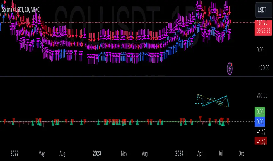
Gann + Laplace Smoothed Hybrid Volume Spread AnalysisThe Gann + Laplace Smoothed Hybrid Volume Spread Analysis ( GannLSHVSA ) Strategy/Indicator is an trading tool designed to fuse volume analysis with trend detection, offering traders a view of market dynamics.
This Strategy/Indicator stands apart by integrating the principles of the upgraded Discrete Fourier Transform (DFT), the Laplace Stieltjes Transform and volume spread analysis, enhanced with a layer of Fourier smoothing to distill market noise and highlight trend directions with unprecedented clarity.
The length of EMA and Strategy Entries are modified with the Gann swings .
This smoothing process allows traders to discern the true underlying patterns in volume and price action, stripped of the distractions of short-term fluctuations and noise.
The core functionality of the GannLSHVSA revolves around the innovative combination of volume change analysis, spread determination (calculated from the open and close price difference), and the strategic use of the EMA (default 10) to fine-tune the analysis of spread by incorporating volume changes.
Trend direction is validated through a moving average (MA) of the histogram, which acts analogously to the Volume MA found in traditional volume indicators. This MA serves as a pivotal reference point, enabling traders to confidently engage with the market when the histogram's movement concurs with the trend direction, particularly when it crosses the Trend MA line, signalling optimal entry points.
It returns 0 when MA of the histogram and EMA of the Price Spread are not align.
WHAT IS GannLSHVSA INDICATOR:
The GannLSHVSA plots a positive trend when a positive Volume smoothed Spread and EMA of Volume smoothed price is above 0, and a negative when negative Volume smoothed Spread and EMA of Volume smoothed price is below 0. When this conditions are not met it plots 0.
HOW TO USE THE STRATEGY:
Here you fine-tune the inputs until you find a combination that works well on all Timeframes you will use when creating your Automated Trade Algorithmic Strategy. I suggest 4h, 12h, 1D, 2D, 3D, 4D, 5D, 6D, W and M.
ORIGINALITY & USEFULNESS:
The GannLSHVSA Strategy is unique because it applies upgraded DFT, the Laplace Stieltjes Transform for data smoothing, effectively filtering out the minor fluctuations and leaving traders with a clear picture of the market's true movements. The DFT's ability to break down market signals into constituent frequencies offers a granular view of market dynamics, highlighting the amplitude and phase of each frequency component. This, combined with the strategic application of Ehler's Universal Oscillator principles via a histogram, furnishes traders with a nuanced understanding of market volatility and noise levels, thereby facilitating more informed trading decisions. The Gann swing strategy is developed by meomeo105, this Gann high and low algorithm forms the basis of the EMA modification.
DETAILED DESCRIPTION:
My detailed description of the indicator and use cases which I find very valuable.
What is the meaning of price spread?
In finance, a spread refers to the difference between two prices, rates, or yields. One of the most common types is the bid-ask spread, which refers to the gap between the bid (from buyers) and the ask (from sellers) prices of a security or asset.
We are going to use Open-Close spread.
What is Volume spread analysis?
Volume spread analysis (VSA) is a method of technical analysis that compares the volume per candle, range spread, and closing price to determine price direction.
What does this mean?
We need to have a positive Volume Price Spread and a positive Moving average of Volume price spread for a positive trend. OR via versa a negative Volume Price Spread and a negative Moving average of Volume price spread for a negative trend.
What if we have a positive Volume Price Spread and a negative Moving average of Volume Price Spread?
It results in a neutral, not trending price action.
Thus the Indicator/Strategy returns 0 and Closes all long and short positions.
I suggest using "Close all" input False when fine-tuning Inputs for 1 TimeFrame. When you export data to Excel/Numbers/GSheets I suggest using "Close all" input as True, except for the lowest TimeFrame. I suggest using 100% equity as your default quantity for fine-tune purposes. I have to mention that 100% equity may lead to unrealistic backtesting results. Be avare. When backtesting for trading purposes use Contracts or USDT.
Fine-tune Inputs: Gann + Laplace Smooth Volume Zone OscillatorUse this Strategy to Fine-tune inputs for the GannLSVZ0 Indicator.
Strategy allows you to fine-tune the indicator for 1 TimeFrame at a time; cross Timeframe Input fine-tuning is done manually after exporting the chart data.
I suggest using "Close all" input False when fine-tuning Inputs for 1 TimeFrame. When you export data to Excel/Numbers/GSheets I suggest using "Close all" input as True, except for the lowest TimeFrame.
MEANINGFUL DESCRIPTION:
The Volume Zone oscillator breaks up volume activity into positive and negative categories. It is positive when the current closing price is greater than the prior closing price and negative when it's lower than the prior closing price. The resulting curve plots through relative percentage levels that yield a series of buy and sell signals, depending on level and indicator direction.
The Gann Laplace Smoothed Volume Zone Oscillator GannLSVZO is a refined version of the Volume Zone Oscillator, enhanced by the implementation of the upgraded Discrete Fourier Transform, the Laplace Stieltjes Transform. Its primary function is to streamline price data and diminish market noise, thus offering a clearer and more precise reflection of price trends.
By combining the Laplace with Gann Swing Entries and with Ehler's white noise histogram, users gain a comprehensive perspective on volume-related market conditions.
HOW TO USE THE INDICATOR:
The default period is 2 but can be adjusted after backtesting. (I suggest 5 VZO length and NoiceR max length 8 as-well)
The VZO points to a positive trend when it is rising above the 0% level, and a negative trend when it is falling below the 0% level. 0% level can be adjusted in setting by adjusting VzoDifference. Oscillations rising below 0% level or falling above 0% level result in a natural trend.
HOW TO USE THE STRATEGY:
Here you fine-tune the inputs until you find a combination that works well on all Timeframes you will use when creating your Automated Trade Algorithmic Strategy. I suggest 4h, 12h, 1D, 2D, 3D, 4D, 5D, 6D, W and M.
When Indicator/Strategy returns 0 or natural trend, Strategy Closes All it's positions.
ORIGINALITY & USFULLNESS:
Personal combination of Gann swings and Laplace Stieltjes Transform of a price which results in less noise Volume Zone Oscillator.
The Laplace Stieltjes Transform is a mathematical technique that transforms discrete data from the time domain into its corresponding representation in the frequency domain. This process involves breaking down a signal into its individual frequency components, thereby exposing the amplitude and phase characteristics inherent in each frequency element.
This indicator utilizes the concept of Ehler's Universal Oscillator and displays a histogram, offering critical insights into the prevailing levels of market noise. The Ehler's Universal Oscillator is grounded in a statistical model that captures the erratic and unpredictable nature of market movements. Through the application of this principle, the histogram aids traders in pinpointing times when market volatility is either rising or subsiding.
The Gann swing strategy is developed by meomeo105, this Gann high and low algorithm forms the basis of the EMA modification.
DETAILED DESCRIPTION:
My detailed description of the indicator and use cases which I find very valuable.
What is oscillator?
Oscillators are chart indicators that can assist a trader in determining overbought or oversold conditions in ranging (non-trending) markets.
What is volume zone oscillator?
Price Zone Oscillator measures if the most recent closing price is above or below the preceding closing price.
Volume Zone Oscillator is Volume multiplied by the 1 or -1 depending on the difference of the preceding 2 close prices and smoothed with Exponential moving Average.
What does this mean?
If the VZO is above 0 and VZO is rising. We have a bullish trend. Most likely.
If the VZO is below 0 and VZO is falling. We have a bearish trend. Most likely.
Rising means that VZO on close is higher than the previous day.
Falling means that VZO on close is lower than the previous day.
What if VZO is falling above 0 line?
It means we have a high probability of a bearish trend.
Thus the indicator returns 0 and Strategy closes all it's positions when falling above 0 (or rising bellow 0) and we combine higher and lower timeframes to gauge the trend.
What is approximation and smoothing?
They are mathematical concepts for making a discrete set of numbers a
continuous curved line.
Laplace Stieltjes Transform approximation of a close price are taken from aprox library.
Key Features:
You can tailor the Indicator/Strategy to your preferences with adjustable parameters such as VZO length, noise reduction settings, and smoothing length.
Volume Zone Oscillator (VZO) shows market sentiment with the VZO, enhanced with Exponential Moving Average (EMA) smoothing for clearer trend identification.
Noise Reduction leverages Euler's White noise capabilities for effective noise reduction in the VZO, providing a cleaner and more accurate representation of market dynamics.
Choose between the traditional Fast Laplace Stieltjes Transform (FLT) and the innovative Double Discrete Fourier Transform (DTF32) soothed price series to suit your analytical needs.
Use dynamic calculation of Laplace coefficient or the static one. You may modify those inputs and Strategy entries with Gann swings.
I suggest using "Close all" input False when fine-tuning Inputs for 1 TimeFrame. When you export data to Excel/Numbers/GSheets I suggest using "Close all" input as True, except for the lowest TimeFrame. I suggest using 100% equity as your default quantity for fine-tune purposes. I have to mention that 100% equity may lead to unrealistic backtesting results. Be avare. When backtesting for trading purposes use Contracts or USDT.

ICT IPDA Liquidity Matrix By AlgoCadosThe ICT IPDA Liquidity Matrix by AlgoCados is a sophisticated trading tool that integrates the principles of the Interbank Price Delivery Algorithm (IPDA), as taught by The Inner Circle Trader (ICT). This indicator is meticulously designed to support traders in identifying key institutional levels and liquidity zones, enhancing their trading strategies with data-driven insights. Suitable for both day traders and swing traders, the tool is optimized for high-frequency and positional trading, providing a robust framework for analyzing market dynamics across multiple time horizons.
# Key Features
Multi-Time Frame Analysis
High Time Frame (HTF) Levels : The indicator tracks critical trading levels over multiple days, specifically at 20, 40, and 60-day intervals. This functionality is essential for identifying long-term trends and significant support and resistance levels that aid in strategic decision-making for swing traders and positional traders.
Low Time Frame (LTF) Levels : It monitors price movements within 20, 40, and 60-hour intervals on lower time frames. This granularity provides a detailed view of intraday price actions, which is crucial for scalping and short-term trading strategies favored by day traders.
Daily Open Integration : The indicator includes the daily opening price, providing a crucial reference point that reflects the market's initial sentiment. This feature helps traders assess the market's direction and volatility, enabling them to make informed decisions based on the day's early movements, which is particularly useful for day trading strategies.
IPDA Reference Points : By leveraging IPDA's 20, 40, and 60-period lookbacks, the tool identifies Key Highs and Lows, which are used by IPDA as Draw On Liquidity. IPDA is an electronic and algorithmic system engineered for achieving price delivery efficiency, as taught by ICT. These reference points serve as benchmarks for understanding institutional trading behavior, allowing traders to align their strategies with the dominant market forces and recognize institutional key levels.
Dynamic Updates and Overlap Management : The indicator is updated daily at the beginning of a new daily candle with the latest market data, ensuring that traders operate with the most current information. It also features intelligent overlap management that prioritizes the most relevant levels based on the timeframe hierarchy, reducing visual clutter and enhancing chart readability.
Comprehensive Customization Options : Traders can tailor the indicator to their specific needs through an extensive input menu. This includes toggles for visibility, line styles, color selections, and label display preferences. These customization options ensure that the tool can adapt to various trading styles and preferences, enhancing user experience and analytical capabilities.
User-Friendly Interface : The tool is designed with a user-friendly interface that includes clear, concise labels for all significant levels. It supports various font families and sizes, making it easier to interpret and act upon the displayed data, ensuring that traders can focus on making informed trading decisions without being overwhelmed by unnecessary information.
# Usage Note
The indicator is segmented into two key functionalities:
LTF Displays : The Low Time Frame (LTF) settings are exclusive to timeframes up to 1 hour, providing detailed analysis for intraday traders. This is crucial for traders who need precise and timely data to make quick decisions within the trading day.
HTF Displays : The High Time Frame (HTF) settings apply to the daily timeframe and any shorter intervals, allowing for comprehensive analysis over extended periods. This is beneficial for swing traders looking to identify broader trends and market directions.
# Inputs and Configurations
BINANCE:BTCUSDT
Offset: Adjustable setting to shift displayed data horizontally for better visibility, allowing traders to view past levels and make informed decisions based on historical data.
Label Styles: Choose between compact or verbose label formats for different levels, offering flexibility in how much detail is displayed on the chart.
Daily Open Line: Customizable line style and color for the daily opening price, providing a clear visual reference for the start of the trading day.
HTF Levels: Configurable high and low lines for HTF with options for style and color customization, allowing traders to highlight significant levels in a way that suits their trading style.
LTF Levels: Similar customization options for LTF levels, ensuring flexibility in how data is presented, making it easier for traders to focus on the most relevant intraday levels.
Text Utils: Settings for font family, size, and text color, allowing for personalized display preferences and ensuring that the chart is both informative and aesthetically pleasing.
# Advanced Features
Overlap Management : The script intelligently handles overlapping levels, particularly where multiple timeframes intersect, by prioritizing the more significant levels and removing redundant ones. This ensures that the charts remain clear and focused on the most critical data points, allowing traders to concentrate on the most relevant market information.
Real-Time Updates : The indicator updates its calculations at the start of each new daily bar, incorporating the latest market data to provide timely and accurate trading signals. This real-time updating is crucial for traders who rely on up-to-date information to execute their strategies effectively and make informed trading decisions.
# Example Use Cases
Scalpers/Day traders: Can utilize the LTF features to make rapid decisions based on hourly market movements, identifying short-term trading opportunities with precision.
Swing Traders: Will benefit from the HTF analysis to identify broader trends and key levels that influence longer-term market movements, enabling them to capture significant market swings.
By providing a clear, detailed view of key market dynamics, the ICT IPDA Liquidity Matrix by AlgoCados empowers traders to make more informed and effective trading decisions, aligning with institutional trading methodologies and enhancing their market understanding.
# Usage Disclaimer
This tool is designed to assist in trading decisions, but it should be used in conjunction with other analysis methods and risk management strategies. Trading involves significant risk, and it is essential to understand the market conditions thoroughly before making trading decisions.

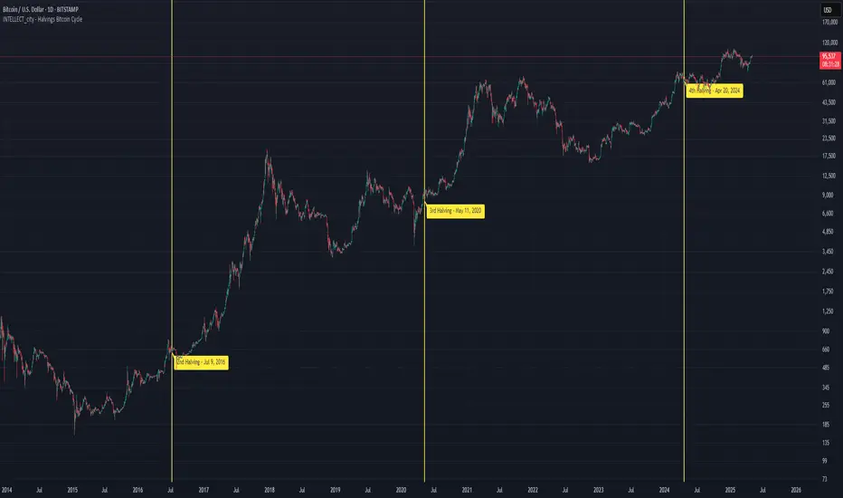
Intellect_city - Halvings Bitcoin CycleWhat is halving?
The halving timer shows when the next Bitcoin halving will occur, as well as the dates of past halvings. This event occurs every 210,000 blocks, which is approximately every 4 years. Halving reduces the emission reward by half. The original Bitcoin reward was 50 BTC per block found.
Why is halving necessary?
Halving allows you to maintain an algorithmically specified emission level. Anyone can verify that no more than 21 million bitcoins can be issued using this algorithm. Moreover, everyone can see how much was issued earlier, at what speed the emission is happening now, and how many bitcoins remain to be mined in the future. Even a sharp increase or decrease in mining capacity will not significantly affect this process. In this case, during the next difficulty recalculation, which occurs every 2014 blocks, the mining difficulty will be recalculated so that blocks are still found approximately once every ten minutes.
How does halving work in Bitcoin blocks?
The miner who collects the block adds a so-called coinbase transaction. This transaction has no entry, only exit with the receipt of emission coins to your address. If the miner's block wins, then the entire network will consider these coins to have been obtained through legitimate means. The maximum reward size is determined by the algorithm; the miner can specify the maximum reward size for the current period or less. If he puts the reward higher than possible, the network will reject such a block and the miner will not receive anything. After each halving, miners have to halve the reward they assign to themselves, otherwise their blocks will be rejected and will not make it to the main branch of the blockchain.
The impact of halving on the price of Bitcoin
It is believed that with constant demand, a halving of supply should double the value of the asset. In practice, the market knows when the halving will occur and prepares for this event in advance. Typically, the Bitcoin rate begins to rise about six months before the halving, and during the halving itself it does not change much. On average for past periods, the upper peak of the rate can be observed more than a year after the halving. It is almost impossible to predict future periods because, in addition to the reduction in emissions, many other factors influence the exchange rate. For example, major hacks or bankruptcies of crypto companies, the situation on the stock market, manipulation of “whales,” or changes in legislative regulation.
---------------------------------------------
Table - Past and future Bitcoin halvings:
---------------------------------------------
Date: Number of blocks: Award:
0 - 03-01-2009 - 0 block - 50 BTC
1 - 28-11-2012 - 210000 block - 25 BTC
2 - 09-07-2016 - 420000 block - 12.5 BTC
3 - 11-05-2020 - 630000 block - 6.25 BTC
4 - 20-04-2024 - 840000 block - 3.125 BTC
5 - 24-03-2028 - 1050000 block - 1.5625 BTC
6 - 26-02-2032 - 1260000 block - 0.78125 BTC
7 - 30-01-2036 - 1470000 block - 0.390625 BTC
8 - 03-01-2040 - 1680000 block - 0.1953125 BTC
9 - 07-12-2043 - 1890000 block - 0.09765625 BTC
10 - 10-11-2047 - 2100000 block - 0.04882813 BTC
11 - 14-10-2051 - 2310000 block - 0.02441406 BTC
12 - 17-09-2055 - 2520000 block - 0.01220703 BTC
13 - 21-08-2059 - 2730000 block - 0.00610352 BTC
14 - 25-07-2063 - 2940000 block - 0.00305176 BTC
15 - 28-06-2067 - 3150000 block - 0.00152588 BTC
16 - 01-06-2071 - 3360000 block - 0.00076294 BTC
17 - 05-05-2075 - 3570000 block - 0.00038147 BTC
18 - 08-04-2079 - 3780000 block - 0.00019073 BTC
19 - 12-03-2083 - 3990000 block - 0.00009537 BTC
20 - 13-02-2087 - 4200000 block - 0.00004768 BTC
21 - 17-01-2091 - 4410000 block - 0.00002384 BTC
22 - 21-12-2094 - 4620000 block - 0.00001192 BTC
23 - 24-11-2098 - 4830000 block - 0.00000596 BTC
24 - 29-10-2102 - 5040000 block - 0.00000298 BTC
25 - 02-10-2106 - 5250000 block - 0.00000149 BTC
26 - 05-09-2110 - 5460000 block - 0.00000075 BTC
27 - 09-08-2114 - 5670000 block - 0.00000037 BTC
28 - 13-07-2118 - 5880000 block - 0.00000019 BTC
29 - 16-06-2122 - 6090000 block - 0.00000009 BTC
30 - 20-05-2126 - 6300000 block - 0.00000005 BTC
31 - 23-04-2130 - 6510000 block - 0.00000002 BTC
32 - 27-03-2134 - 6720000 block - 0.00000001 BTC
Gaussian Price Filter [BackQuant]Gaussian Price Filter
Overview and History of the Gaussian Transformation
The Gaussian transformation, often associated with the Gaussian (normal) distribution, is a mathematical function characteristically prominent in statistics and probability theory. The bell-shaped curve of the Gaussian function, expressing the normal distribution, is ubiquitously employed in various scientific and engineering disciplines, including financial market analysis. This transformation's core utility in trading and economic forecasting is derived from its efficacy in smoothing data series and highlighting underlying trends, which are pivotal for making strategic trading decisions.
The Gaussian filter, specifically, is a type of data-smoothing algorithm that mitigates the random "noise" of market price data, thus enhancing the visibility of crucial trend changes and patterns. Historically, this concept was adapted from fields such as signal processing and image editing, where precise extraction of useful information from noisy environments is critical.
1. What is a Gaussian Transformation?
A Gaussian transformation involves the application of a Gaussian function to a set of data points. The function is applied as a filter in the context of trading algorithms to smooth time series data, which helps in identifying the intrinsic trends obscured by market volatility. The transformation is characterized by its parameter, sigma (σ), representing the standard deviation, which determines the width of the Gaussian bell curve. The breadth of this curve impacts the degree of smoothing: a wider curve (higher sigma value) results in more smoothing, beneficial for longer-term trend analysis.
2. Filtering Price with Gaussian Transformation and its Benefits
In the provided Script, the Gaussian transformation is utilized to filter price data. The filtering process involves convolving the price data with Gaussian weights, which are calculated based on the chosen length (the number of data points considered) and sigma. This convolution process smooths out short-term fluctuations and highlights longer-term movements, facilitating a clearer analysis of market trends.
Benefits:
Reduces noise: It filters out minor price movements and random fluctuations, which are often misleading.
Enhances trend recognition: By smoothing the data, it becomes easier to identify significant trends and reversals.
Improves decision-making: Traders can make more informed decisions by focusing on substantive, smoothed data rather than reacting to random noise.
3. Potential Limitations and Issues
While Gaussian filters are highly effective in smoothing data, they are not without limitations:
Lag introduction: Like all moving averages, the Gaussian filter introduces a lag between the actual price movements and the output signal, which can delay decision-making.
Feature blurring: Over-smoothing might obscure significant price movements, especially if a large sigma is used.
Parameter sensitivity: The choice of length and sigma significantly affects the output, requiring optimization and backtesting to determine the best settings for specific market conditions.
4. Extending Gaussian Filters to Other Indicators
The methodology used to filter price data with a Gaussian filter can similarly be applied to other technical indicators, such as RSI (Relative Strength Index) or MACD (Moving Average Convergence Divergence). By smoothing these indicators, traders can reduce false signals and enhance the reliability of the indicators' outputs, leading to potentially more accurate signals and better timing for entering or exiting trades.
5. Application in Trading
In trading, the Gaussian Price Filter can be strategically used to:
Spot trend reversals: Smoothed price data can more clearly indicate when a trend is starting to change, which is crucial for catching reversals early.
Define entry and exit points: The filtered data points can help in setting more precise entry and exit thresholds, minimizing the risk and maximizing the potential return.
Filter other data streams: Apply the Gaussian filter on volume or open interest data to identify significant changes in market dynamics.
6. Functionality of the Script
The script is designed to:
Calculate Gaussian weights (f_gaussianWeights function): Generates the weights used for the Gaussian kernel based on the provided length and sigma.
Apply the Gaussian filter (f_applyGaussianFilter function): Uses the weights to compute the smoothed price data.
Conditional Trend Detection and Coloring: Determines the trend direction based on the filtered price and colors the price bars on the chart to visually represent the trend.
7. Specific Actions of This Code
The Pine Script provided by BackQuant executes several specific actions:
Input Handling: It allows users to specify the source data (src), kernel length, and sigma directly in the chart settings.
Weight Calculation and Normalization: Computes the Gaussian weights and normalizes them to ensure their sum equals one, which maintains the original data scale.
Filter Application: Applies the normalized Gaussian kernel to the price data to produce a smoothed output.
Trend Identification and Visualization: Identifies whether the market is trending upwards or downwards based on the smoothed data and colors the bars green (up) or red (down) to indicate the trend direction.

Momentum Ghost Machine [ChartPrime]Momentum Ghost Machine (ChartPrime) is designed to be the next generation in momentum/rate of change analysis. This indicator utilizes the properties of one of our favorite filters to create a more accurate and stable momentum oscillator by using a high quality filtered delayed signal to do the momentum comparison.
Traditional momentum/roc uses the raw price data to compare current price to previous price to generate a directional oscillator. This leaves the oscillator prone to false readings and noisy outputs that leave traders unsure of the real likelihood of a future movement. One way to mitigate this issue would be to use some sort of moving average. Unfortunately, this can only go so far because simple moving average algorithms result in a poor reconstruction of the actual shape of the underlying signal.
The windowed sinc low pass filter is a linear phase filter, meaning that it doesn't change the shape or size of the original signal when applied. This results in a faithful reconstruction of the original signal, but without the "high frequency noise". Just like any filter, the process of applying it requires that we have "future" samples resulting in a time delay for real time applications. Fortunately this is a great thing in the context of a momentum oscillator because we need some representation of past price data to compare the current price data to. By using an ideal low pass filter to generate this delayed signal we can super charge the momentum oscillator and fix the majority of issues its predecessors had.
This indicator has a few extra features that other momentum/roc indicators dont have. One major yet simple improvement is the inclusion of a moving average to help gauge the rate of change of this indicator. Since we included a moving average, we thought it would only be appropriate to add a histogram to help visualize the relationship between the signal and its average. To go further with this we have also included linear extrapolation to further help you predict the momentum and direction of this oscillator. Included with this extrapolation we have also added the histogram in the extrapolation to further enhance its visual interpretation. Finally, the inclusion of a candle coloring feature really drives how the utility of the Momentum Machine .
There are three distinct options when using the candle coloring feature: Direct, MA, and Both. With direct the candles will be colored based on the indicators direction and polarity. When it is above zero and moving up, it displays a green color. When it is above zero and moving down it will display a light green color. Conversely, when the indicator is below zero and moving down it displays a red color, and when it it moving up and below zero it will display a light red color. MA coloring will color the candles just like a MACD. If the signal is above its MA and moving up it will display a green color, and when it is above its MA and moving down it will display a light green color.
When the signal is below its MA and moving down it will display a red color, and when its below its ma and moving up it will display a light red color. Both combines the two into a single color scheme providing you with the best of both worlds. If the indicator is above zero it will display the MA colors with a slight twist. When the indicator is moving down and is below its MA it will display a lighter color than before, and when it is below zero and is above its MA it will display a darker color color.
Length of 50 with a smoothing of 100
Length of 50 with a smoothing of 25
By default, the indicator is set to a momentum length of 50, with a post smoothing of 2. We have chosen the longer period for the momentum length to highlight the performance of this indicator compared to its ancestors. A major point to consider with this indicator is that you can only achieve so much smoothing for a chosen delay. This is because more data is required to produce a smoother signal at a specified length. Once you have selected your desired momentum length you can then select your desired momentum smoothing . This is made possible by the use of the windowed sinc low pass algorithm because it includes a frequency cutoff argument. This means that you can have as little or as much smoothing as you please without impacting the period of the indicator. In the provided examples above this paragraph is a visual representation of what is going on under the hood of this indicator. The blue line is the filtered signal being compared to the current closing price. As you can see, the filtered signal is very smooth and accurately represents the underlying price action without noise.
We hope that users can find the same utility as we did in this indicator and that it levels up your analysis utilizing the momentum oscillator or rate of change.
Enjoy
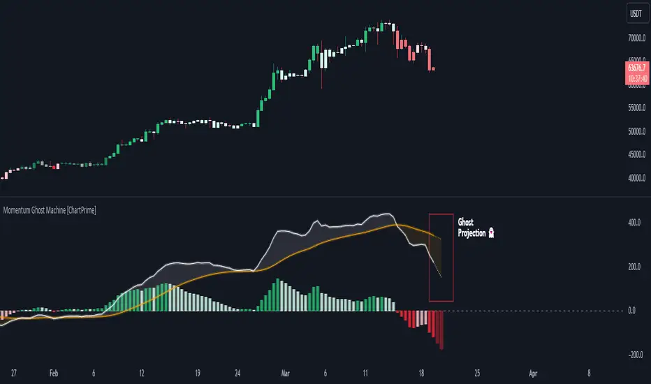
Kalman Price Filter [BackQuant]Kalman Price Filter
The Kalman Filter, named after Rudolf E. Kálmán, is a algorithm used for estimating the state of a linear dynamic system from a series of noisy measurements. Originally developed for aerospace applications in the early 1960s, such as guiding Apollo spacecraft to the moon, it has since been applied across numerous fields including robotics, economics, and, notably, financial markets. Its ability to efficiently process noisy data in real-time and adapt to new measurements has made it a valuable tool in these areas.
Use Cases in Financial Markets
1. Trend Identification:
The Kalman Filter can smooth out market price data, helping to identify the underlying trend amidst the noise. This is particularly useful in algorithmic trading, where identifying the direction and strength of a trend can inform trade entry and exit decisions.
2. Market Prediction:
While no filter can predict the future with certainty, the Kalman Filter can be used to forecast short-term market movements based on current and historical data. It does this by estimating the current state of the market (e.g., the "true" price) and projecting it forward under certain model assumptions.
3. Risk Management:
The Kalman Filter's ability to estimate the volatility (or noise) of the market can be used for risk management. By dynamically adjusting to changes in market conditions, it can help traders adjust their position sizes and stop-loss orders to better manage risk.
4. Pair Trading and Arbitrage:
In pair trading, where the goal is to capitalize on the price difference between two correlated securities, the Kalman Filter can be used to estimate the spread between the pair and identify when the spread deviates significantly from its historical average, indicating a trading opportunity.
5. Optimal Asset Allocation:
The filter can also be applied in portfolio management to dynamically adjust the weights of different assets in a portfolio based on their estimated risks and returns, optimizing the portfolio's performance over time.
Advantages in Financial Applications
Adaptability: The Kalman Filter continuously updates its estimates with each new data point, making it well-suited to markets that are constantly changing.
Efficiency: It processes data and updates estimates in real-time, which is crucial for high-frequency trading strategies.
Handling Noise: Its ability to distinguish between the signal (e.g., the true price trend) and noise (e.g., random fluctuations) is particularly valuable in financial markets, where price data can be highly volatile.
Challenges and Considerations
Model Assumptions: The effectiveness of the Kalman Filter in financial applications depends on the accuracy of the model used to describe market dynamics. Financial markets are complex and influenced by numerous factors, making model selection critical.
Parameter Sensitivity: The filter's performance can be sensitive to the choice of parameters, such as the process and measurement noise values. These need to be carefully selected and potentially adjusted over time.
Despite these challenges, the Kalman Filter remains a potent tool in the quantitative trader's arsenal, offering a sophisticated method to extract useful information from noisy financial data. Its use in trading strategies should, however, be complemented with sound risk management practices and an awareness of the limitations inherent in any model-based approach to trading.

Exponentially Weighted Moving Average Oscillator [BackQuant]Exponentially Weighted Moving Average (EWMA)
The Exponentially Weighted Moving Average (EWMA) is a quantitative or statistical measure used to model or describe a time series. The EWMA is widely used in finance, the main applications being technical analysis and volatility modeling.
The moving average is designed as such that older observations are given lower weights. The weights fall exponentially as the data point gets older – hence the name exponentially weighted.
Applications of the EWMA
The EWMA is widely used in technical analysis. It may not be used directly, but it is used in conjunction with other indicators to generate trading signals. A well-known example is the Negative Volume Index (NVI), which is used in conjunction with its EWMA.
Why is it different from the In-Built TradingView EWMA
Adaptive Algorithms: If your strategy requires the alpha parameter to change adaptively based on certain conditions (for example, based on market volatility), a for loop can be used to adjust the weights dynamically within the loop as opposed to the fixed decay rate in the standard EWMA.
Customization: A for loop allows for more complex and nuanced calculations that may not be directly supported by built-in functions. For example, you might want to adjust the weights in a non-standard way that the typical EWMA calculation doesn't allow for.
Use of the Oscillator
This mainly comes from 3 main premises, this is something I like to do personally since it is easier to work with them in the context of my system. E.g. Using them to spot clear trends without noise on longer timeframes.
Clarity: Plotting the EWMA as an oscillator provides a clear visual representation of the momentum or trend strength. It allows traders to see overbought or oversold conditions relative to a normalized range.
Comparison: An oscillator can make it easier to compare different securities or timeframes on a similar scale, especially when normalized. This is because the oscillator values are typically bounded within a range (like -1 to 1 or 0 to 100), whereas the actual price series can vary significantly.
Focus on Change: When plotted as an oscillator, the focus is on the rate of change or the relative movement of the EWMA, not on the absolute price levels. This can help traders spot divergences or convergences that may not be as apparent when the EWMA is plotted directly on the price chart. This is also one reason there is a conditional plotting on the chart.
Trend Strength: When normalized, the distance of the oscillator from its midpoint can be interpreted as the strength of the trend, providing a quantitative measure that can be used to make systematic trading decisions.
Here are the backtests on the 1D Timeframe for
BITSTAMP:BTCUSD
BITSTAMP:ETHUSD
COINBASE:SOLUSD
When using this script the user is able to define a source and period, which by extension calculates the alpha. An option to colour the bars accord to trend.
This makes it super easy to use in a system.
I recommend using this as above the midline (0) for a positive trend and below the midline for negative trend.
Hence why I put a label on the last bar to ensure it is easier for traders to read.
Lastly, The decreasing colour relative to RoC, this also helps traders to understand the strength of the indicator and gain insight into when to potentially reduce position size.
This indicator is best used in the medium timeframe.

Squeeze Momentum DeluxeThe Squeeze Momentum Deluxe is a comprehensive trading toolkit built with features of momentum, volatility, and price action. This script offers a suite for both mean reversion and trend-following analysis. Developed based on the original TTM Squeeze implementation by @LazyBear, this indicator introduces several innovative components to enhance your trading insights.
🔲 Components and Features
Momentum Oscillator - as rooted in the TTM Squeeze, quantifies the relationship between price and its extremes over a defined period. By normalizing the calculation, the values become comparable throughout time and across securities, allowing for a nuanced assessment of Bullish and Bearish momentum. Furthermore, by presenting it as a ribbon with a signal line we gain additional information about the direction of price swings.
Squeeze Bars - The original squeeze concept is based on the relationship between the Bollinger Bands and Keltner Channel , once the BB resides inside the KC a squeeze occurs. By understanding their fundamentals a new form of calculation can be inferred.
method bb(float src, simple int len, simple float mult) => method kc(float src, simple int len, simple float mult) =>
float basis = ta.sma (src, len) float basis = ta.sma (src, len)
float dev = ta.stdev(src, len) float rng = ta.atr ( len)
float upper = basis + dev * mult float upper = basis + rng * mult
float lower = basis - dev * mult float lower = basis - rng * mult
Both BB and KC are constructed upon a moving average with the addition of Standard Deviation and Average True Range respectively. Therefore, the calculation can be transformed to when the Stdev is lower than the ATR a squeeze occurs.
method sqz(float src, simple int len) =>
float dev = ta.stdev(src, len)
float atr = ta.atr ( len)
dev < atr ? true : false
This indicator uses three different thresholds for the ATR to gain three levels of price "Squeeze" for further analysis.
Directional Flux- This component measures the overall direction of price volatility, offering insights into trend sentiment. Presented as waves in the background, it includes an OverFlux feature to signal extreme market bias in a particular direction which can signal either exhaustion or vital continuation. Additionally, the user can choose if to base the calculation on Heikin-Ashi Candles to bias the tool toward trend assessment.
Confluence Gauges - Placed at the top and bottom of the indicator, these gauges measure confluence in the relationship between the Momentum Oscillator and Directional Flux. They provide traders with an easily interpretable visual aid for detecting market sentiment. Reversal doritos displayed alongside them contribute to mean reversion analysis.
Divergences (Real-Time) - Equipped with a custom algorithm, the indicator detects real-time divergences between price and the oscillator. This dynamic feature enhances your ability to spot potential trend reversals as they occur.
🔲 Settings
Directional Flux Length - Adjusts the period of which the background volatility waves operate on.
Trend Bias - Bases the calculation of the Flux to HA candles to bias its behavior toward the trend of price action.
Squeeze Momentum Length - Calibrates the length of the main oscillator ribbon as well as the period for the squeeze algorithm.
Signal - Controls the width of the ribbon. Lower values result in faster responsiveness at the cost of premature positives.
Divergence Sensitivity - Adjusts a threshold to limit the amount of divergences detected based on strength. Higher values result in less detections, stronger structure.
🔲 Alerts
Sell Signal
Buy Signal
Bullish Momentum
Bearish Momentum
Bullish Flux
Bearish Flux
Bullish Swing
Bearish Swing
Strong Bull Gauge
Strong Bear Gauge
Weak Bull Gauge
Weak Bear Gauge
High Squeeze
Normal Squeeze
Low Squeeze
Bullish Divergence
Bearish Divergence
As well as the option to trigger 'any alert' call.
The Squeeze Momentum Deluxe is a comprehensive tool that goes beyond traditional momentum indicators, offering a rich set of features to elevate your trading strategy. I recommend using toolkit alongside other indicators to have a wide variety of confluence to therefore gain higher probabilistic and better informed decisions.

LIT - Timings Fx MartinThe Asia Liquidity Points Indicator is a powerful tool designed for traders to identify key liquidity points during the Asia trading session. This script is tailored specifically to aid traders in capitalizing on the unique characteristics of Asian markets, providing invaluable insights into liquidity zones that can significantly enhance trading decisions.
Key Features:
Asia Session Focus: The indicator focuses exclusively on the Asia trading session, which encompasses the trading activity primarily in the Asian markets such as Tokyo, Hong Kong, Singapore, and others.
Liquidity Zones Identification: The script utilizes advanced algorithms to identify and map out liquidity zones within the Asia trading session. These zones represent areas where significant buying or selling pressure is likely to occur, thus presenting lucrative trading opportunities.
Customizable Parameters: Traders have the flexibility to customize various parameters such as time frame, sensitivity, and display options to suit their trading preferences and strategies.
Visual Alerts: The indicator provides visual alerts on the trading chart, clearly indicating the location and strength of liquidity points. This feature enables traders to quickly identify potential entry or exit points based on the liquidity dynamics in the market.
Real-Time Updates: The script continuously monitors market activity during the Asia session, providing real-time updates on liquidity points as they evolve. This ensures traders stay informed and adaptable to changing market conditions.
Integration with Trading Strategies: The Asia Liquidity Points Indicator seamlessly integrates with various trading strategies, serving as a valuable tool for both discretionary and algorithmic traders. Whether used in isolation or in combination with other technical analysis tools, this indicator can enhance trading performance and profitability.
User-Friendly Interface: The indicator boasts a user-friendly interface, making it accessible to traders of all levels of experience. Whether you are a novice trader or a seasoned professional, you can easily incorporate this tool into your trading arsenal.
In conclusion, the Asia Liquidity Points Indicator offers traders a strategic advantage in navigating the nuances of the Asia trading session. By identifying key liquidity zones and providing real-time insights, this script empowers traders to make informed decisions and capitalize on lucrative trading opportunities in the dynamic Asian markets.
Order Blocks Finder [TradingFinder] Major OB | Supply and Demand🔵 Introduction
Drawing all order blocks on the path, especially in range-bound or channeling markets, fills the chart with lines, making it confusing rather than providing the trader with the best entry and exit points.
🔵 Reason for Indicator Creation
For traders familiar with market structure and only need to know the main accumulation points (best entry or exit points), and primary order blocks that act as strong sources of power.
🟣 Important Note
All order blocks, both ascending and descending, are identified and displayed on the chart when the structure of "BOS" or "CHOCH" is broken, which can also be identified with "MSS."
🔵 How to Use
When the indicator is installed, it plots all order blocks (active order blocks) and continues until the price reaches them. This continuation happens in boxes to have a better view in the TradingView chart.
Green Range : Ascending order blocks where we expect a price increase in these areas.
Red Range : Descending order blocks where we expect a price decrease in these areas.
🔵 Settings
Order block refine setting : When Order block refine is off, the supply and demand zones are the entire length of the order block (Low to High) in their standard state and cannot be improved. If you turn on Order block refine, supply and demand zones will improve using the error correction algorithm.
Refine type setting : Improving order blocks using the error correction algorithm can be done in two ways: Defensive and Aggressive. In the Aggressive method, the largest possible range is considered for order blocks.
🟣 Important
The main advantage of the Aggressive method is minimizing the loss of stops, but due to the widening of the supply or demand zone, the reward-to-risk ratio decreases significantly. The Aggressive method is suitable for individuals who take high-risk trades.
In the Defensive method, the range of order blocks is minimized to their standard state. In this case, fewer stops are triggered, and the reward-to-risk ratio is maximized in its optimal state. It is recommended for individuals who trade with low risk.
Show high level setting : If you want to display major high levels, set show high level to Yes.
Show low level setting : If you want to display major low levels, set show low level to Yes.
🔵 How to Use
The general view of this indicator is as follows.
When the price approaches the range, wait for the price reaction to confirm it, such as a pin bar or divergence.
If the price passes with a strong candle (spike), especially after a long-range or at the beginning of sessions, a powerful event is happening, and it is outside the credibility level.
An Example of a Valid Zone
An Example of Breakout and Invalid Zone. (My suggestion is not to use pending orders, especially when the market is highly volatile or before and after news.)
After reaching this zone, expect the price to move by at least the minimum candle that confirmed it or a price ceiling or floor.
🟣 Important : These factors can be more accurately measured with other trend finder indicators provided.
🔵 Auxiliary Tools
There is much talk about not using trend lines, candlesticks, Fibonacci, etc., in the web space. However, our suggestion is to create and use tools that can help you profit from this market.
• Fibonacci Retracement
• Trading Sessions
• Candlesticks
🔵 Advantages
• Plotting main OBs without additional lines;
• Suitable for timeframes M1, M5, M15, H1, and H4;
• Effective in Tokyo, Sydney, and London sessions;
• Plotting the main ceiling and floor to help identify the trend.
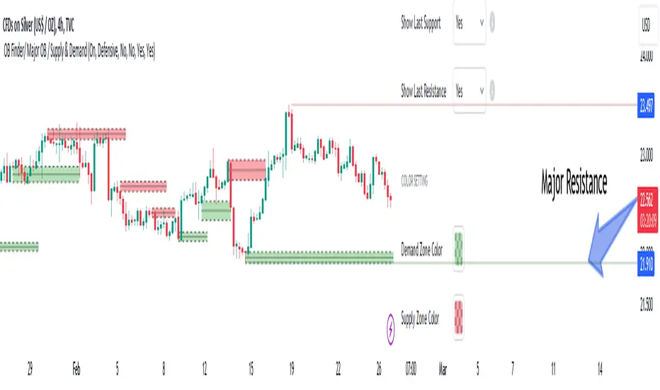
ATR Range Accumulation by Standard Deviation and Volume [SS]So, this is an indicator/premise I have been experimenting with, which mixes ATR with Z-Score and Volume metrics.
What does the indicator do?
The indicator, on the lower timeframes, uses an ATR approach to determine short-term ranges. It takes the average ATR range over a designated lookback period and plots out the levels like so:
It then calculates the Z-Score for these ATR targets (shown in the chart above) and calculates, over the designated lookback period, how often price accumulates at that standard deviation level.
The indicator is essentially a hybrid of my Z-Score Support and Resistance indicator and my frequency distribution indicator. It combines both concepts into one.
You also have the option of sorting by volume accumulation. This will display the accumulation of the ranges by volume accumulation, like so:
Larger Timeframes:
If you want to see the accumulation by volume or standard deviation on the larger timeframes, you can. Simply toggle on your preferred setting:
Show Total Accumulation Breakdown:
This will break down the levels, over the lookback period, by standard deviation. This is similar to the Z-Score support and resistance indicator. It will then show you how often price accumulates at these various standard deviation levels. Here is an example on the daily timeframe using the 1D chart settings:
Inversely, you can repeat this, with the Z-Score levels, but show accumulation by volume. This will print 5 boxes, which are between +3 Standard Deviations and -3 Standard Deviations, like so:
Here we can see that 61% of volume accumulation is between -1 and 1 standard deviation.
Using it to Trade:
For swing trading, I suggest using the larger timeframe information. However, for both swing and day traders, it is also helpful to use the ATR display. You can modify the ATR display to show the levels on any timeframe by selecting which timeframe you would like to see ATR ranges for. If you are trading on the 1 or 5-minute chart, I suggest leaving the levels at no shorter than a 60-minute timeframe.
You can also use these levels on the daily for the weekly levels, etc.
The accumulation being shown will be based on the current chart timeframe. This is a function of Pinescript, but in this case, it's actually advantageous because if you are trading on the shorter timeframe, and a level has 0% recent accumulation, it's unlikely we will see that level soon or overly quickly. Intraday retracements will generally happen to areas of high accumulation.
How this indicator is different:
The difference in this indicator comes from its focus on accumulation in relation to Standard Deviation. There is one thing that is consistent among retail traders, algorithms, market makers, and funds, and that is looking at the market in terms of standard deviation. Each person, market maker, and algorithm may be slightly nuanced in how it conceptualizes standard deviation (whether it be since the inception of the ticker (or IPO), or the previous 500 days, or the previous 100 days, etc.), but the premise remains consistent. Standard Deviation is a really important, if not the most important, metric to pay attention to. Another important metric is volume. Thus, the premise is that combining volume accumulation with standard deviation should, theoretically, be telling. We can see the extent of buying at various standard deviations and whether a stock is really a buy or not.
And that's the indicator! Hope you enjoy it. Leave your comments and questions below.
Safe trades!