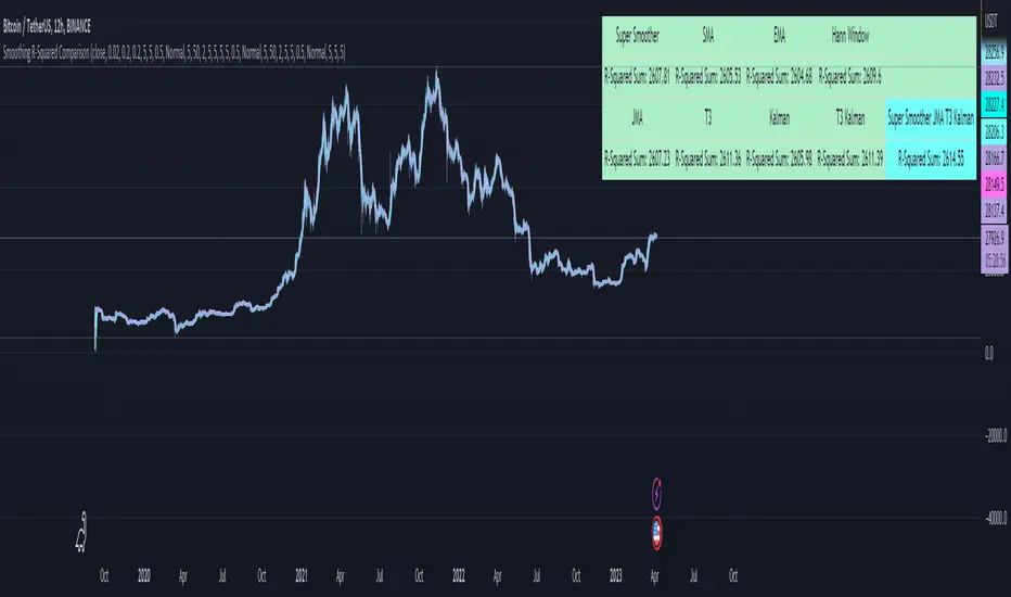
Smoothing R-Squared ComparisonIntroduction
Heyo guys, here I made a comparison between my favorised smoothing algorithms.
I chose the R-Squared value as rating factor to accomplish the comparison.
The indicator is non-repainting.
Description
In technical analysis, traders often use moving averages to smooth out the noise in price data and identify trends. While moving averages are a useful tool, they can also obscure important information about the underlying relationship between the price and the smoothed price.
One way to evaluate this relationship is by calculating the R-squared value, which represents the proportion of the variance in the price that can be explained by the smoothed price in a linear regression model.
This PineScript code implements a smoothing R-squared comparison indicator.
It provides a comparison of different smoothing techniques such as Kalman filter, T3, JMA, EMA, SMA, Super Smoother and some special combinations of them.
The Kalman filter is a mathematical algorithm that uses a series of measurements observed over time, containing statistical noise and other inaccuracies, and produces estimates of unknown variables that tend to be more accurate than those based on a single measurement.
The input parameters for the Kalman filter include the process noise covariance and the measurement noise covariance, which help to adjust the sensitivity of the filter to changes in the input data.
The T3 smoothing technique is a popular method used in technical analysis to remove noise from a signal.
The input parameters for the T3 smoothing method include the length of the window used for smoothing, the type of smoothing used (Normal or New), and the smoothing factor used to adjust the sensitivity to changes in the input data.
The JMA smoothing technique is another popular method used in technical analysis to remove noise from a signal.
The input parameters for the JMA smoothing method include the length of the window used for smoothing, the phase used to shift the input data before applying the smoothing algorithm, and the power used to adjust the sensitivity of the JMA to changes in the input data.
The EMA and SMA techniques are also popular methods used in technical analysis to remove noise from a signal.
The input parameters for the EMA and SMA techniques include the length of the window used for smoothing.
The indicator displays a comparison of the R-squared values for each smoothing technique, which provides an indication of how well the technique is fitting the data.
Higher R-squared values indicate a better fit. By adjusting the input parameters for each smoothing technique, the user can compare the effectiveness of different techniques in removing noise from the input data.
Usage
You can use it to find the best fitting smoothing method for the timeframe you usually use.
Just apply it on your preferred timeframe and look for the highlighted table cell.
Conclusion
It seems like the T3 works best on timeframes under 4H.
There's where I am active, so I will use this one more in the future.
Thank you for checking this out. Enjoy your day and leave me a like or comment. 🧙♂️
---
Credits to:
▪@loxx – T3
▪@balipour – Super Smoother
▪ChatGPT – Wrote 80 % of this article and helped with the research
Buscar en scripts para "algo"
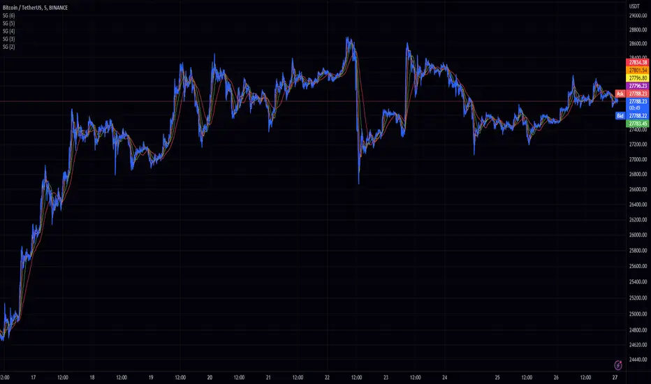
Spectral Gating (SG)The Spectral Gating (SG) Indicator is a technical analysis tool inspired by music production techniques. It aims to help traders reduce noise in their charts by focusing on the significant frequency components of the data, providing a clearer view of market trends.
By incorporating complex number operations and Fast Fourier Transform (FFT) algorithms, the SG Indicator efficiently processes market data. The indicator transforms input data into the frequency domain and applies a threshold to the power spectrum, filtering out noise and retaining only the frequency components that exceed the threshold.
Key aspects of the Spectral Gating Indicator include:
Adjustable Window Size: Customize the window size (ranging from 2 to 6) to control the amount of data considered during the analysis, giving you the flexibility to adapt the indicator to your trading strategy.
Complex Number Arithmetic: The indicator uses complex number addition, subtraction, and multiplication, as well as radius calculations for accurate data processing.
Iterative FFT and IFFT: The SG Indicator features iterative FFT and Inverse Fast Fourier Transform (IFFT) algorithms for rapid data analysis. The FFT algorithm converts input data into the frequency domain, while the IFFT algorithm restores the filtered data back to the time domain.
Spectral Gating: At the heart of the indicator, the spectral gating function applies a threshold to the power spectrum, suppressing frequency components below the threshold. This process helps to enhance the clarity of the data by reducing noise and focusing on the more significant frequency components.
Visualization: The indicator plots the filtered data on the chart with a simple blue line, providing a clean and easily interpretable representation of the results.
Although the Spectral Gating Indicator may not be a one-size-fits-all solution for all trading scenarios, it serves as a valuable tool for traders looking to reduce noise and concentrate on relevant market trends. By incorporating this indicator into your analysis toolkit, you can potentially make more informed trading decisions.
PSv5 3D Array/Matrix Super Hack"In a world of ever pervasive and universal deceit, telling a simple truth is considered a revolutionary act."
INTRO:
First, how about a little bit of philosophic poetry with another dimension applied to it?
The "matrix of control" is everywhere...
It is all around us, even now in the very place you reside. You can see it when you look at your digitized window outwards into the world, or when you turn on regularly scheduled television "programs" to watch news narratives and movies that subliminally influence your thoughts, feelings, and emotions. You have felt it every time you have clocked into dead end job workplaces... when you unknowingly worshiped on the conformancy alter to cultish ideologies... and when you pay your taxes to a godvernment that is poisoning you softly and quietly by injecting your mind and body with (psyOps + toxicCompounds). It is a fictitiously generated world view that has been pulled over your eyes to blindfold, censor, and mentally prostrate you from spiritually hearing the real truth.
What TRUTH you must wonder? That you are cognitively enslaved, like everyone else. You were born into mental bondage, born into an illusory societal prison complex that you are entirely incapable of smelling, tasting, or touching. Its a contrived monetary prison enterprise for your mind and eternal soul, built by pretending politicians, corporate CONartists, and NonGoverning parasitic Organizations deploying any means of infiltration and deception by using every tactic unimaginable. You are slowly being convinced into becoming a genetically altered cyborg by acclimation, socially engineered and chipped to eventually no longer be 100% human.
Unfortunately no one can be told eloquently enough in words what the matrix of control truly is. You have to experience it and witness it for yourself. This is your chance to program a future paradigm that doesn't yet exist. After visiting here, there is absolutely no turning back. You can continually take the blue pill BIGpharmacide wants you to repeatedly intake. The story ends if you continually sleep walk through a 2D hologram life, believing whatever you wish to believe until you cease to exist. OR, you can take the red pill challenge, explore "question every single thing" wonderland, program your arse off with 3D capabilities, ultimately ascertaining a new mathematical empyrean. Only then can you fully awaken to discover how deep the rabbit hole state of affairs transpire worldwide with a genuine open mind.
Remember, all I'm offering is a mathematical truth, nothing more...
PURPOSE:
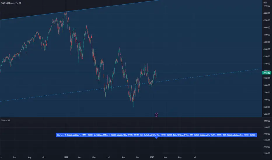
With that being said above, it is now time for advanced developers to start creating their own matrix constructs in 3D, in Pine, just as the universe is created spatially. For those of you who instantly know what this script's potential is easily capable of, you already know what you have to do with it. While this is simplistically just a 3D array for either integers or floats, additional companion functions can in the future be constructed by other members to provide a more complete matrix/array library for millions of folks on TV. I do encourage the most courageous of mathemagicians on TV to do so. I have been employing very large 2D/3D array structures for quite some time, and their utility seems to be of great benefit. Discovering that for myself, I fully realized that Pine is incomplete and must be provided with this agility to process complex datasets that traders WILL use in the future. Mark my words!
CONCEPTION:
While I have long realized and theorized this code for a great duration of time, I was finally able to turn it into a Pine reality with the assistance and training of an "artificially intuitive" program while probing its aptitude. Even though it knows virtually nothing about Pine Script 4.0 or 5.0 syntax, functions, and behavior, I was able to conjure code into an identity similar to what you see now within a few minutes. Close enough for me! Many manual edits later for pine compliance, and I had it in chart, presto!
While most people consider the service to be an "AI", it didn't pass my Pine Turing test. I did have to repeatedly correct it, suffered through numerous apologies from it, was forced to use specifically tailored words, and also rationally debate AND argued with it. It is a handy helper but beware of generating Pine code from it, trust me on this one. However... this artificially intuitive service is currently available in its infancy as version 3. Version 4 most likely will have more diversity to enhance my algorithmic expertise of Pine wizardry. I do have to thank E.M. and his developers for an eye opening experience, or NONE of this code below would be available as you now witness it today.
LIMITATIONS:
As of this initial release, Pine only supports 100,000 array elements maximum. For example, when using this code, a 50x50x40 element configuration will exceed this limit, but 50x50x39 will work. You will always have to keep that in mind during development. Running that size of an array structure on every single bar will most likely time out within 20-40 seconds. This is not the most efficient method compared to a real native 3D array in action. Ehlers adepts, this might not be 100% of what you require to "move forward". You can try, but head room with a low ceiling currently will be challenging to walk in for now, even with extremely optimized Pine code.
A few common functions are provided, but this can be extended extensively later if you choose to undertake that endeavor. Use the code as is and/or however you deem necessary. Any TV member is granted absolute freedom to do what they wish as they please. I ultimately wish to eventually see a fully equipped library version for both matrix3D AND array3D created by collaborative efforts that will probably require many Pine poets testing collectively. This is just a bare bones prototype until that day arrives. Considerably more computational server power will be required also. Anyways, I hope you shall find this code somewhat useful.
Notice: Unfortunately, I will not provide any integration support into members projects at all. I have my own projects that require too much of my time already.
POTENTIAL APPLICATIONS:
The creation of very large coefficient 3D caches/buffers specifically at bar_index==0 can dramatically increase runtime agility for thousands of bars onwards. Generating 1000s of values once and just accessing those generated values is much faster. Also, when running dozens of algorithms simultaneously, a record of performance statistics can be kept, self-analyzed, and visually presented to the developer/user. And, everything else under the sun can be created beyond a developers wildest dreams...
EPILOGUE:
Free your mind!!! And unleash weapons of mass financial creation upon the earth for all to utilize via the "Power of Pine". Flying monkeys and minions are waging economic sabotage upon humanity, decimating markets and exchanges. You can always see it your market charts when things go horribly wrong. This is going to be an astronomical technical challenge to continually navigate very choppy financial markets that are increasingly becoming more and more unstable and volatile. Ordinary one plot algorithms simply are not enough anymore. Statistics and analysis sits above everything imagined. This includes banking, godvernment, corporations, REAL science, technology, health, medicine, transportation, energy, food, etc... We have a unique perspective of the world that most people will never get to see, depending on where you look. With an ever increasingly complex world in constant dynamic flux, novel ways to process data intricately MUST emerge into existence in order to tackle phenomenal tasks required in the future. Achieving data analysis in 3D forms is just one lonely step of many more to come.
At this time the WesternEconomicFraudsters and the WorldHealthOrders are attempting to destroy/reset the world's financial status in order to rain in chaos upon most nations, causing asset devaluation and hyper-inflation. Every form of deception, infiltration, and theft is occurring with a result of destroyed wealth in preparation to consolidate it. Open discussions, available to the public, by world leaders/moguls are fantasizing about new dystopian system as a one size fits all nations solution of digitalID combined with programmableDemonicCurrencies to usher in a new form of obedient servitude to a unipolar digitized hegemony of monetary vampires. If they do succeed with economic conquest, as they have publicly stated, people will be converted into human cattle, herded within smart cities, you will own nothing, eat bugs for breakfast/lunch/dinner, live without heat during severe winter conditions, and be happy. They clearly haven't done the math, as they are far outnumbered by a ratio of 1 to millions. Sith Lords do not own planet Earth! The new world disorder of human exploitation will FAIL. History, my "greatest teacher" for decades reminds us over, and over, and over again, and what are time series for anyways? They are for an intense mathematical analysis of prior historical values/conditions in relation to today's values/conditions... I imagine one day we will be able to ask an all-seeing AI, "WHO IS TO BLAME AND WHY AND WHEN?" comprised of 300 pages in great detail with images, charts, and statistics.
What are the true costs of malignant lies? I will tell you... 64bit numbers are NOT even capable of calculating the extreme cost of pernicious lies and deceit. That's how gigantic this monstrous globalization problem has become and how awful the "matrix of control" truly is now. ALL nations need a monumental revision of its CODE OF ETHICS, and that's definitely a multi-dimensional problem that needs solved sooner than later. If it was up to me, economies and technology would be developed so extensively to eliminate scarcity and increase the standard of living so high, that the notion of war and conflict would be considered irrelevant and extremely appalling to the future generations of humanity, our grandchildren born and unborn. The future will not be owned and operated by geriatric robber barons destined to expire quickly. The future will most likely be intensely "guided" by intelligent open source algorithms that youthful generations will inherit as their birth right.
P.S. Don't give me that politco-my-diction crap speech below in comments. If they weren't meddling with economics mucking up 100% of our chart results in 100% of tickers, I wouldn't have any cause to analyze any effects generated by them, nor provide this script's code. I am performing my analytical homework, but have you? Do you you know WHY international affairs are in dire jeopardy? Without why, the "Power of Pine" would have never existed as it specifically does today. I'm giving away much of my mental power generously to TV members so you are specifically empowered beyond most mathematical agilities commonly existing. I'm just a messenger of profound ideas. Loving and loathing of words is ALWAYS in the eye of beholders, and that's why the freedom of speech is enshrined as #1 in the constitutional code of the USA. Without it, this entire site might not have been allowed to exist from its founder's inceptions.
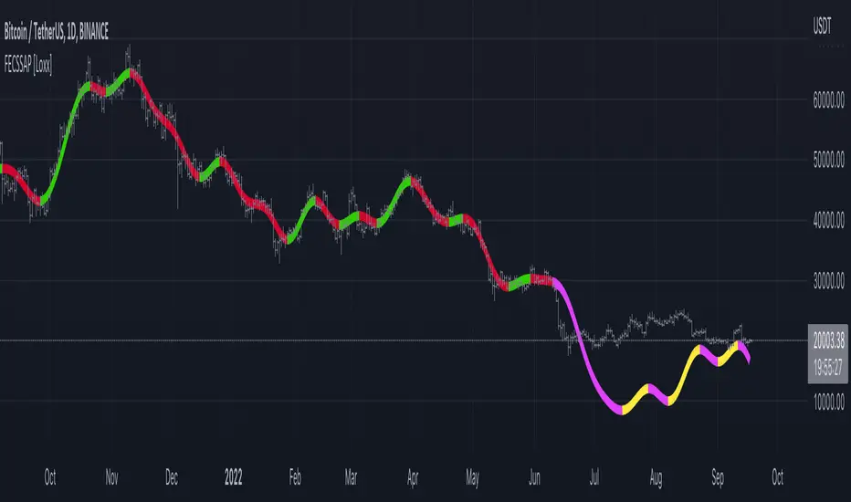
Fourier Extrapolator of 'Caterpillar' SSA of Price [Loxx]Fourier Extrapolator of 'Caterpillar' SSA of Price is a forecasting indicator that applies Singular Spectrum Analysis to input price and then injects that transformed value into the Quinn-Fernandes Fourier Transform algorithm to generate a price forecast. The indicator plots two curves: the green/red curve indicates modeled past values and the yellow/fuchsia dotted curve indicates the future extrapolated values.
What is the Fourier Transform Extrapolator of price?
Fourier Extrapolator of Price is a multi-harmonic (or multi-tone) trigonometric model of a price series xi, i=1..n, is given by:
xi = m + Sum( a*Cos(w*i) + b*Sin(w*i), h=1..H )
Where:
xi - past price at i-th bar, total n past prices;
m - bias;
a and b - scaling coefficients of harmonics;
w - frequency of a harmonic ;
h - harmonic number;
H - total number of fitted harmonics.
Fitting this model means finding m, a, b, and w that make the modeled values to be close to real values. Finding the harmonic frequencies w is the most difficult part of fitting a trigonometric model. In the case of a Fourier series, these frequencies are set at 2*pi*h/n. But, the Fourier series extrapolation means simply repeating the n past prices into the future.
Quinn-Fernandes algorithm find sthe harmonic frequencies. It fits harmonics of the trigonometric series one by one until the specified total number of harmonics H is reached. After fitting a new harmonic , the coded algorithm computes the residue between the updated model and the real values and fits a new harmonic to the residue.
see here: A Fast Efficient Technique for the Estimation of Frequency , B. G. Quinn and J. M. Fernandes, Biometrika, Vol. 78, No. 3 (Sep., 1991), pp . 489-497 (9 pages) Published By: Oxford University Press
Fourier Transform Extrapolator of Price inputs are as follows:
npast - number of past bars, to which trigonometric series is fitted;
nharm - total number of harmonics in model;
frqtol - tolerance of frequency calculations.
What is Singular Spectrum Analysis ( SSA )?
Singular spectrum analysis ( SSA ) is a technique of time series analysis and forecasting. It combines elements of classical time series analysis, multivariate statistics, multivariate geometry, dynamical systems and signal processing. SSA aims at decomposing the original series into a sum of a small number of interpretable components such as a slowly varying trend, oscillatory components and a ‘structureless’ noise. It is based on the singular value decomposition ( SVD ) of a specific matrix constructed upon the time series. Neither a parametric model nor stationarity-type conditions have to be assumed for the time series. This makes SSA a model-free method and hence enables SSA to have a very wide range of applicability.
For our purposes here, we are only concerned with the "Caterpillar" SSA . This methodology was developed in the former Soviet Union independently (the ‘iron curtain effect’) of the mainstream SSA . The main difference between the main-stream SSA and the "Caterpillar" SSA is not in the algorithmic details but rather in the assumptions and in the emphasis in the study of SSA properties. To apply the mainstream SSA , one often needs to assume some kind of stationarity of the time series and think in terms of the "signal plus noise" model (where the noise is often assumed to be ‘red’). In the "Caterpillar" SSA , the main methodological stress is on separability (of one component of the series from another one) and neither the assumption of stationarity nor the model in the form "signal plus noise" are required.
"Caterpillar" SSA
The basic "Caterpillar" SSA algorithm for analyzing one-dimensional time series consists of:
Transformation of the one-dimensional time series to the trajectory matrix by means of a delay procedure (this gives the name to the whole technique);
Singular Value Decomposition of the trajectory matrix;
Reconstruction of the original time series based on a number of selected eigenvectors.
This decomposition initializes forecasting procedures for both the original time series and its components. The method can be naturally extended to multidimensional time series and to image processing.
The method is a powerful and useful tool of time series analysis in meteorology, hydrology, geophysics, climatology and, according to our experience, in economics, biology, physics, medicine and other sciences; that is, where short and long, one-dimensional and multidimensional, stationary and non-stationary, almost deterministic and noisy time series are to be analyzed.
"Caterpillar" SSA inputs are as follows:
lag - How much lag to introduce into the SSA algorithm, the higher this number the slower the process and smoother the signal
ncomp - Number of Computations or cycles of of the SSA algorithm; the higher the slower
ssapernorm - SSA Period Normalization
numbars =- number of past bars, to which SSA is fitted
Included:
Bar coloring
Alerts
Signals
Loxx's Expanded Source Types
Related Fourier Transform Indicators
Real-Fast Fourier Transform of Price w/ Linear Regression
Fourier Extrapolator of Variety RSI w/ Bollinger Bands
Fourier Extrapolator of Price w/ Projection Forecast
Related Projection Forecast Indicators
Itakura-Saito Autoregressive Extrapolation of Price
Helme-Nikias Weighted Burg AR-SE Extra. of Price
Related SSA Indicators
End-pointed SSA of FDASMA
End-pointed SSA of Williams %R
Levinson-Durbin Autocorrelation Extrapolation of Price [Loxx]Levinson-Durbin Autocorrelation Extrapolation of Price is an indicator that uses the Levinson recursion or Levinson–Durbin recursion algorithm to predict price moves. This method is commonly used in speech modeling and prediction engines.
What is Levinson recursion or Levinson–Durbin recursion?
Is a linear algebra prediction analysis that is performed once per bar using the autocorrelation method with a within a specified asymmetric window. The autocorrelation coefficients of the window are computed and converted to LP coefficients using the Levinson algorithm. The LP coefficients are then transformed to line spectrum pairs for quantization and interpolation. The interpolated quantized and unquantized filters are converted back to the LP filter coefficients to construct the synthesis and weighting filters for each bar.
Data inputs
Source Settings: -Loxx's Expanded Source Types. You typically use "open" since open has already closed on the current active bar
LastBar - bar where to start the prediction
PastBars - how many bars back to model
LPOrder - order of linear prediction model; 0 to 1
FutBars - how many bars you want to forward predict
Things to know
Normally, a simple moving average is caculated on source data. I've expanded this to 38 different averaging methods using Loxx's Moving Avreages.
This indicator repaints
Included
Bar color muting
Further reading
Implementing the Levinson-Durbin Algorithm on the StarCore™ SC140/SC1400 Cores
LevinsonDurbin_G729 Algorithm, Calculates LP coefficients from the autocorrelation coefficients. Intel® Integrated Performance Primitives for Intel® Architecture Reference Manual

APA-Adaptive, Ehlers Early Onset Trend [Loxx]APA-Adaptive, Ehlers Early Onset Trend is Ehlers Early Onset Trend but with Autocorrelation Periodogram Algorithm dominant cycle period input.
What is Ehlers Early Onset Trend?
The Onset Trend Detector study is a trend analyzing technical indicator developed by John F. Ehlers , based on a non-linear quotient transform. Two of Mr. Ehlers' previous studies, the Super Smoother Filter and the Roofing Filter, were used and expanded to create this new complex technical indicator. Being a trend-following analysis technique, its main purpose is to address the problem of lag that is common among moving average type indicators.
The Onset Trend Detector first applies the EhlersRoofingFilter to the input data in order to eliminate cyclic components with periods longer than, for example, 100 bars (default value, customizable via input parameters) as those are considered spectral dilation. Filtered data is then subjected to re-filtering by the Super Smoother Filter so that the noise (cyclic components with low length) is reduced to minimum. The period of 10 bars is a default maximum value for a wave cycle to be considered noise; it can be customized via input parameters as well. Once the data is cleared of both noise and spectral dilation, the filter processes it with the automatic gain control algorithm which is widely used in digital signal processing. This algorithm registers the most recent peak value and normalizes it; the normalized value slowly decays until the next peak swing. The ratio of previously filtered value to the corresponding peak value is then quotiently transformed to provide the resulting oscillator. The quotient transform is controlled by the K coefficient: its allowed values are in the range from -1 to +1. K values close to 1 leave the ratio almost untouched, those close to -1 will translate it to around the additive inverse, and those close to zero will collapse small values of the ratio while keeping the higher values high.
Indicator values around 1 signify uptrend and those around -1, downtrend.
What is an adaptive cycle, and what is Ehlers Autocorrelation Periodogram Algorithm?
From his Ehlers' book Cycle Analytics for Traders Advanced Technical Trading Concepts by John F. Ehlers , 2013, page 135:
"Adaptive filters can have several different meanings. For example, Perry Kaufman’s adaptive moving average ( KAMA ) and Tushar Chande’s variable index dynamic average ( VIDYA ) adapt to changes in volatility . By definition, these filters are reactive to price changes, and therefore they close the barn door after the horse is gone.The adaptive filters discussed in this chapter are the familiar Stochastic , relative strength index ( RSI ), commodity channel index ( CCI ), and band-pass filter.The key parameter in each case is the look-back period used to calculate the indicator. This look-back period is commonly a fixed value. However, since the measured cycle period is changing, it makes sense to adapt these indicators to the measured cycle period. When tradable market cycles are observed, they tend to persist for a short while.Therefore, by tuning the indicators to the measure cycle period they are optimized for current conditions and can even have predictive characteristics.
The dominant cycle period is measured using the Autocorrelation Periodogram Algorithm. That dominant cycle dynamically sets the look-back period for the indicators. I employ my own streamlined computation for the indicators that provide smoother and easier to interpret outputs than traditional methods. Further, the indicator codes have been modified to remove the effects of spectral dilation.This basically creates a whole new set of indicators for your trading arsenal."

Jurik Composite Fractal Behavior (CFB) on EMA [Loxx]Jurik Composite Fractal Behavior (CFB) on EMA is an exponential moving average with adaptive price trend duration inputs. This purpose of this indicator is to introduce the formulas for the calculation Composite Fractal Behavior. As you can see from the chart above, price reacts wildly to shifts in volatility--smoothing out substantially while riding a volatility wave and cutting sharp corners when volatility drops. Notice the chop zone on BTC around August 2021, this was a time of extremely low relative volatility.
This indicator uses three previous indicators from my public scripts. These are:
JCFBaux Volatility
Jurik Filter
Jurik Volty
The CFB is also related to the following indicator
Jurik Velocity ("smoother moment")
Now let's dive in...
What is Composite Fractal Behavior (CFB)?
All around you mechanisms adjust themselves to their environment. From simple thermostats that react to air temperature to computer chips in modern cars that respond to changes in engine temperature, r.p.m.'s, torque, and throttle position. It was only a matter of time before fast desktop computers applied the mathematics of self-adjustment to systems that trade the financial markets.
Unlike basic systems with fixed formulas, an adaptive system adjusts its own equations. For example, start with a basic channel breakout system that uses the highest closing price of the last N bars as a threshold for detecting breakouts on the up side. An adaptive and improved version of this system would adjust N according to market conditions, such as momentum, price volatility or acceleration.
Since many systems are based directly or indirectly on cycles, another useful measure of market condition is the periodic length of a price chart's dominant cycle, (DC), that cycle with the greatest influence on price action.
The utility of this new DC measure was noted by author Murray Ruggiero in the January '96 issue of Futures Magazine. In it. Mr. Ruggiero used it to adaptive adjust the value of N in a channel breakout system. He then simulated trading 15 years of D-Mark futures in order to compare its performance to a similar system that had a fixed optimal value of N. The adaptive version produced 20% more profit!
This DC index utilized the popular MESA algorithm (a formulation by John Ehlers adapted from Burg's maximum entropy algorithm, MEM). Unfortunately, the DC approach is problematic when the market has no real dominant cycle momentum, because the mathematics will produce a value whether or not one actually exists! Therefore, we developed a proprietary indicator that does not presuppose the presence of market cycles. It's called CFB (Composite Fractal Behavior) and it works well whether or not the market is cyclic.
CFB examines price action for a particular fractal pattern, categorizes them by size, and then outputs a composite fractal size index. This index is smooth, timely and accurate
Essentially, CFB reveals the length of the market's trending action time frame. Long trending activity produces a large CFB index and short choppy action produces a small index value. Investors have found many applications for CFB which involve scaling other existing technical indicators adaptively, on a bar-to-bar basis.
What is Jurik Volty used in the Juirk Filter?
One of the lesser known qualities of Juirk smoothing is that the Jurik smoothing process is adaptive. "Jurik Volty" (a sort of market volatility ) is what makes Jurik smoothing adaptive. The Jurik Volty calculation can be used as both a standalone indicator and to smooth other indicators that you wish to make adaptive.
What is the Jurik Moving Average?
Have you noticed how moving averages add some lag (delay) to your signals? ... especially when price gaps up or down in a big move, and you are waiting for your moving average to catch up? Wait no more! JMA eliminates this problem forever and gives you the best of both worlds: low lag and smooth lines.
Ideally, you would like a filtered signal to be both smooth and lag-free. Lag causes delays in your trades, and increasing lag in your indicators typically result in lower profits. In other words, late comers get what's left on the table after the feast has already begun.
Modifications and improvements
1. Jurik's original calculation for CFB only allowed for depth lengths of 24, 48, 96, and 192. For theoretical purposes, this indicator allows for up to 20 different depth inputs to sample volatility. These depth lengths are
2, 3, 4, 6, 8, 12, 16, 24, 32, 48, 64, 96, 128, 192, 256, 384, 512, 768, 1024, 1536
Including these additional length inputs is arguable useless, but they are are included for completeness of the algorithm.
2. The result of the CFB calculation is forced to be an integer greater than or equal to 1.
3. The result of the CFB calculation is double filtered using an advanced, (and adaptive itself) filtering algorithm called the Jurik Filter. This filter and accompanying internal algorithm are discussed above.

Customizable Non-Repainting HTF MACD MFI Scalper Bot StrategyThis script was originally shared by Wunderbit as a free open source script for the community to work with.
WHAT THIS SCRIPT DOES:
It is intended for use on an algorithmic bot trading platform but can be used for scalping and manual trading.
This strategy is based on the trend-following momentum indicator . It includes the Money Flow index as an additional point for entry.
HOW IT DOES IT:
It uses a combination of MACD and MFI indicators to create entry signals. Parameters for each indicator have been surfaced for user configurability.
Take profits are fixed, but stop loss uses ATR configuration to minimize losses and close profitably.
HOW IS MY VERSION ORIGINAL:
I started trying to deploy this script myself in my algorithmic trading but ran into some issues which I have tried to address in this version.
Delayed Signals : The script has been refactored to use a time frame drop down. The higher time frame can be run on a faster chart (recommended on one minute chart for fastest signal confirmation and relay to algotrading platform.)
Repainting Issues : All indicators have been recoded to use the security function that checks to see if the current calculation is in realtime, if it is, then it uses the previous bar for calculation. If you are still experiencing repainting issues based on intended (or non intended use), please provide a report with screenshot and explanation so I can try to address.
Filtering : I have added to additional filters an ABOVE EMA Filter and a BELOW RSI Filter (both can be turned on and off)
Customizable Long and Close Messages : This allows someone to use the script for algorithmic trading without having to alter code. It also means you can use one indicator for all of your different alterts required for your bots.
HOW TO USE IT:
It is intended to be used in the 5-30 minute time frames, but you might be able to get a good configuration for higher time frames. I welcome feedback from other users on what they have found.
Find a pair with high volatility (example KUCOIN:ETH3LUSDT ) - I have found it works particularly well with 3L and 3S tokens for crypto. although it the limitation is that confrigurations I have found to work typically have low R/R ratio, but very high win rate and profit factor.
Ideally set one minute chart for bots, but you can use other charts for manual trading. The signal will be delayed by one bar but I have found configurations that still test well.
Select a time frame in configuration for your indicator calculations.
Select the strategy config for time frame. I like to use 5 and 15 minutes for scalping scenarios, but I am interested in hearing back from other community memebers.
Optimize your indicator without filters (trendFilter and RSI Filter)
Use the TrendFilter and RSI Filter to further refine your signals for entry. You will get less entries but you can increase your win ratio.
I will add screenshots and possibly a video provided that it passes community standards.
Limitations: this works rather well for short term, and does some good forward testing but back testing large data sets is a problem when switching from very small time frame to large time frame. For instance, finding a configuration that works on a one minute chart but then changing to a 1 hour chart means you lose some of your intra bar calclulations. There are some new features in pine script which might be able to address, this, but I have not had a chance to work on that issue.

Bogdan Ciocoiu - MakaveliDescription
This indicator integrates the functionality of multiple volume price analysis algorithms whilst aligning their scales to fit in a single chart.
Having such indicators loaded enables traders to take advantage of potential divergences between the price action and volume related volatility.
Users will have to enable or disable alternative algorithms depending on their choice.
Uniqueness
This indicator is unique because it combines multiple algorithm-specific two-volume analyses with price volatility.
This indicator is also unique because it amends different algorithms to show output on a similar scale enabling traders to observe various volume-analysis tools simultaneously whilst allocating different colour codes.
Open source re-use
This indicator utilises the following open-source scripts:

Acrypto - Weighted StrategyHello traders!
I have been developing a fully customizable algo over the last year. The algorithm is based on a set of different strategies, each with its own weight (weighted strategy). The set of strategies that I currently use are 5:
MACD
Stochastic RSI
RSI
Supertrend
MA crossover
Moreover, the algo includes STOP losses criteria and a taking profit strategy. The algo must be optimized for the desired asset to achieves its full potential. The 1H and 4H dataframe give good results. The algo has been tested for several asset (same dataframe, different optimization values).
Important note:
Backtest the algorithm with different data stamps to avoid overfitting results
Best,
Alberto

MathSearchDijkstraLibrary "MathSearchDijkstra"
Shortest Path Tree Search Methods using Dijkstra Algorithm.
min_distance(distances, flagged_vertices) Find the lowest cost/distance.
Parameters:
distances : float array, data set with distance costs to start index.
flagged_vertices : bool array, data set with visited vertices flags.
Returns: int, lowest cost/distance index.
dijkstra(matrix_graph, dim_x, dim_y, start) Dijkstra Algorithm, perform a greedy tree search to calculate the cost/distance to selected start node at each vertex.
Parameters:
matrix_graph : int array, matrix holding the graph adjacency list and costs/distances.
dim_x : int, x dimension of matrix_graph.
dim_y : int, y dimension of matrix_graph.
start : int, the vertex index to start search.
Returns: int array, set with costs/distances to each vertex from start vertexs.
shortest_path(start, end, matrix_graph, dim_x, dim_y) Retrieves the shortest path between 2 vertices in a graph using Dijkstra Algorithm.
Parameters:
start : int, the vertex index to start search.
end : int, the vertex index to end search.
matrix_graph : int array, matrix holding the graph adjacency list and costs/distances.
dim_x : int, x dimension of matrix_graph.
dim_y : int, y dimension of matrix_graph.
Returns: int array, set with vertex indices to the shortest path.

P-Square - Estimation of the Nth percentile of a seriesEstimation of the Nth percentile of a series
When working with built-in functions in TradingView we have to limit our length parameters to max 4999. In case we want to use a function on the whole available series (bar 0 all the way to the current bar), we can usually not do this without manually creating these calculations in our code. For things like mean or standard deviation, this is quite trivial, but for things like percentiles, this is usually very costly. In more complex scripts, this becomes impossible because of resource restrictions from the Pine Script execution servers.
One solution to this is to use an estimation algorithm to get close to the true percentile value. Therefore, I have ported this implementation of the P-Square algorithm to Pine Script. P-Square is a fast algorithm that does a good job at estimating percentiles in data streams. Here's the algorithms original paper .
The chart
On the chart we see:
The returns of the series (blue scatter plot)
The mean of the returns of the series (orange line)
The standard deviation of the returns of the series (yellow line)
The actual 84.1th percentile of the returns (white line)
The estimatedl 84.1th percentile of the returns using the P-Square algorithm (green line)
Note: We can see that the returns are not normally distributed as we can see that one standard deviation is higher than the 84.1th percentile. One standard deviation should equal the 84.1th percentile if the data is normally distributed.

Machine Learning: Logistic RegressionMulti-timeframe Strategy based on Logistic Regression algorithm
Description:
This strategy uses a classic machine learning algorithm that came from statistics - Logistic Regression (LR).
The first and most important thing about logistic regression is that it is not a 'Regression' but a 'Classification' algorithm. The name itself is somewhat misleading. Regression gives a continuous numeric output but most of the time we need the output in classes (i.e. categorical, discrete). For example, we want to classify emails into “spam” or 'not spam', classify treatment into “success” or 'failure', classify statement into “right” or 'wrong', classify election data into 'fraudulent vote' or 'non-fraudulent vote', classify market move into 'long' or 'short' and so on. These are the examples of logistic regression having a binary output (also called dichotomous).
You can also think of logistic regression as a special case of linear regression when the outcome variable is categorical, where we are using log of odds as dependent variable. In simple words, it predicts the probability of occurrence of an event by fitting data to a logit function.
Basically, the theory behind Logistic Regression is very similar to the one from Linear Regression, where we seek to draw a best-fitting line over data points, but in Logistic Regression, we don’t directly fit a straight line to our data like in linear regression. Instead, we fit a S shaped curve, called Sigmoid, to our observations, that best SEPARATES data points. Technically speaking, the main goal of building the model is to find the parameters (weights) using gradient descent.
In this script the LR algorithm is retrained on each new bar trying to classify it into one of the two categories. This is done via the logistic_regression function by updating the weights w in the loop that continues for iterations number of times. In the end the weights are passed through the sigmoid function, yielding a prediction.
Mind that some assets require to modify the script's input parameters. For instance, when used with BTCUSD and USDJPY, the 'Normalization Lookback' parameter should be set down to 4 (2,...,5..), and optionally the 'Use Price Data for Signal Generation?' parameter should be checked. The defaults were tested with EURUSD.
Note: TradingViews's playback feature helps to see this strategy in action.
Warning: Signals ARE repainting.
Style tags: Trend Following, Trend Analysis
Asset class: Equities, Futures, ETFs, Currencies and Commodities
Dataset: FX Minutes/Hours/Days

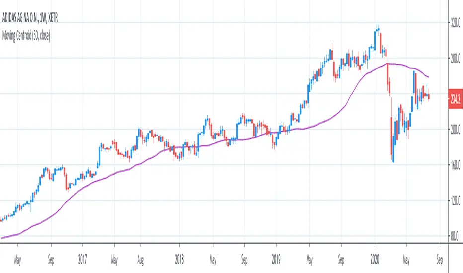
[R&D] Moving CentroidThis script utilizes this concept. Instead of weighting by volume, it weights by amount of price action on every close price of the rolling window. I assume it can be used as an additional reference point for price mode and price antimode.
it is directly connected with Market (not volume) profile, or TPO charts.
The algorithm:
1) takes a rolling window of, for example, 50 data points of close prices:
2) for each of this closing prices, the algorithm will check how many bars touched this close price.
3) then: sum of datapoints * weights/sum of weights
Since the logic is implemented in pretty non-efficient way, the script sometimes can take time to make calculations. Moreover, it calculates the centroid taking into account only close prices, not every tick. of a given rolling window That's why it's still experimental.
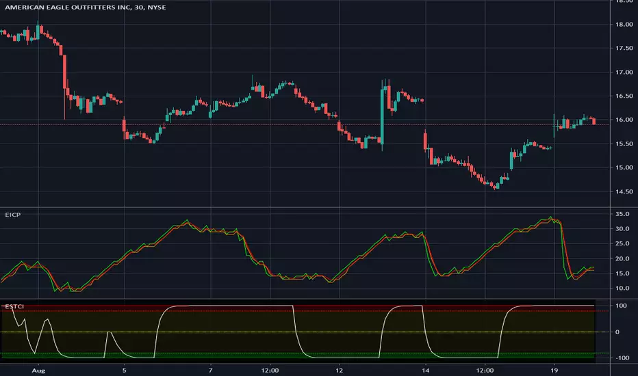
Enhanced Instantaneous Cycle Period - Dr. John EhlersThis is my first public release of detector code entitled "Enhanced Instantaneous Cycle Period" for PSv4.0 I built many months ago. Be forewarned, this is not an indicator, this is a detector to be used by ADVANCED developers to build futuristic indicators in Pine. The origins of this script come from a document by Dr. John Ehlers entitled "SIGNAL ANALYSIS CONCEPTS". You may find this using the NSA's reverse search engine "goggles", as I call it. John Ehlers' MESA used this measurement to establish the data window for analysis for MESA Cycle computations. So... does any developer wish to emulate MESA Cycle now??
I decided to take instantaneous cycle period to another level of novel attainability in this public release of source code with the following methods, if you are curious how I ENHANCED it. Firstly I reduced the delay of accurate measurement from bar_index==0 by quite a few bars closer to IPO. Secondarily, I provided a limit of 6 for a minimum instantaneous cycle period. At bar_index==0, it would provide a period of 0 wrecking many algorithms from the start. I also increased the instantaneous cycle period's maximum value to 80 from 50, providing a window of 6-80 for the instantaneous cycle period value window limits. Thirdly, I replaced the internal EMA with another algorithm. It reduces the lag while extracting a floating point number, for algorithms that will accept that, compared to a sluggish ordinary EMA return. You will see the excessive EMA delay with adding plot(ema(ICP,7)) as it was originally designed. Lastly it's in one simple function for reusability in a nice little package comprising of less than 40 lines of code. I hope I explained that adequately enough and gave you the reader a glimpse of the "Power of Pine" combined with ingenuity.
Be forewarned again, that most of Pine's built-in functions will not accept a floating-point number or dynamic integers for the "length" of it's calculation. You will have to emulate the built-in functions by creating Pine based custom functions, and I assure you, this is very possible in many cases, but not all without array support. You may use int(ICP) to extract an integer from the smoothICP return variable, which may be favorable compared to the choppiness/ringing if ICP alone.
This is commonly what my dense intricate code looks like behind the veil. If you are wondering why there is barely any notation, that's because the notation is in the variable naming and this is intended primarily for ADVANCED developers too. It does contain lines of code that explore techniques in Pine that may be applicable in other Pine projects for those learning or wishing to excel with Pine.
Showcased in the chart below is my free to use "Enhanced Schaff Trend Cycle Indicator", having a common appeal to TV users frequently. If you do have any questions or comments regarding this indicator, I will consider your inquiries, thoughts, and ideas presented below in the comments section, when time provides it. As always, "Like" it if you simply just like it with a proper thumbs up, and also return to my scripts list occasionally for additional postings. Have a profitable future everyone!
NOTICE: Copy pasting bandits who may be having nefarious thoughts, DO NOT attempt this, because this may violate Tradingview's terms, conditions and/or house rules. "WE" are always watching the TV community vigilantly for mischievous behaviors and actions that exploit well intended authors for the purpose of increasing brownie points in reputation scores. Hiding behind a "protected" wall may not protect you from investigation and account penalization by TV staff. Be respectful, and don't just throw an ma() in there branding it as "your" gizmo. Fair enough? Alrighty then... I firmly believe in "innovating" future state-of-the-art indicators, and please contact me if you wish to do so.
FxShare - CC ReversalVery simple , but very grounded, strict and pure math+statistics -based algo:
Based on candle count and reverse .
You can set how many candles (and their body shape) you count in a row before the retracement and market overstretch happens. It also has an EMA filter if you wish for even stronger but more rare signals.
Use it, break it, improve it.

Ranked Exchange Volume (REV)📊 Ranked Exchange Volume (REV) - Multi-Venue Volume Distribution Visualizer
## Stop Guessing Where the Real Volume Is. See It.
Most traders look at aggregate volume and miss the critical story: **where** that volume actually traded. Ranked Exchange Volume (REV) solves this by revealing the complete liquidity landscape across multiple trading venues in a single, elegant visualization.
This isn't just another volume indicator—it's a **dynamic stratified histogram** that automatically reorganizes exchange layers by magnitude on every bar, showing you **instant market dominance** at a glance.
---
## 🎯 The Core Innovation: Self-Organizing Volume Layers
REV displays volume from up to 10 different exchanges as **stacked, color-coded bars** where the largest volume source literally rises to the top. Watch as exchanges compete for dominance in real-time:
- **Largest volume = Top of the bar** (most visible position)
- **Smallest volume = Bottom of the bar** (foundation layer)
- **Everything in between = Automatically sorted on every candle**
This visual hierarchy makes it instantly obvious which venues are leading the market—no mental math required.
---
## ✨ Key Features
### 🔄 **Dynamic Layer Sorting**
Unlike static stacked charts, REV uses real-time stratification. If Binance had 60% of volume last bar but Coinbase takes 70% this bar, you'll see Coinbase jump to the top. The hierarchy reflects current reality, not a fixed order.
### 🎨 **10 Fully Customizable Exchange Slots**
Each exchange slot offers complete control:
- **Enable/Disable toggle** - Turn exchanges on/off without losing your configuration
- **Custom prefix** - Track ANY exchange on TradingView (BINANCE, KRAKEN, OANDA, FXCM, etc.)
- **Custom suffix** - Specify quote currency (USDT, USD, EUR, or leave blank for stocks/forex)
- **Display name** - Control how exchanges appear in the rankings table
- **Color selection** - Match your chart theme or use brand colors for instant recognition
### 📊 **Live Rankings Table**
A real-time leaderboard shows:
- **Rank** - Current position (1 = highest volume)
- **Exchange name** - With color-coded background
- **Volume** - Intelligently formatted with K/M/B units
- **Percentage** - Exact market share
**Table positioning:** Choose from 9 screen positions (top/middle/bottom × left/center/right) to keep your chart clean.
### 🧮 **Intelligent Volume Formatting**
REV automatically detects volume magnitude and applies the appropriate scale:
- **Billions** - Displays as "1.5B" for readability
- **Millions** - Displays as "342.8M"
- **Thousands** - Displays as "45.2K"
- **Full numbers option** - Toggle to see complete values (23,456,789)
The scale adjusts per-bar, so you always see the clearest representation.
### 🚨 **Three Built-In Alert Conditions**
1. **Exchange Dominance Alert (>50%)**
- Triggers when a single venue controls majority of volume
- Signals potential liquidity concentration risk or exchange-specific events
2. **Volume Spike Alert (>2x average)**
- Detects unusual aggregate activity across all venues
- Catches breakouts, news events, or institutional flow
3. **Liquidity Migration Alert**
- Fires when market leadership shifts between exchanges
- Reveals arbitrage opportunities or changing market structure
### 📈 **Optional Total Volume Line**
Display aggregate volume from all exchanges as a reference overlay with customizable color.
---
## 🌍 Market Compatibility: Beyond Crypto
While optimized for cryptocurrency (its primary design), REV works across multiple asset classes:
### ✅ **Cryptocurrency (Perfect Fit)**
**Why it excels:** Crypto trades 24/7 across dozens of global exchanges simultaneously. REV reveals true price discovery.
**Example configurations:**
- **BTC/USDT:** Compare Binance, Coinbase, OKX, Bybit, Kraken, Bitget
- **ETH/USD:** Track institutional venues (Coinbase, Kraken, Gemini) vs retail (Binance, Gate.io)
- **Altcoins:** Identify which exchanges have the deepest liquidity before placing large orders
**Trading applications:**
- **Arbitrage detection** - Spot when volume migrates between venues (price differential opportunities)
- **Exchange risk** - Don't trade on exchanges with suspiciously low volume
- **Whale tracking** - Sudden Coinbase dominance often signals institutional activity
- **Market maker identification** - Consistent Binance leadership suggests MM concentration
### ✅ **Forex (Excellent Fit)**
**Why it works:** Forex doesn't have centralized exchanges—it trades OTC across multiple broker feeds. REV shows which data providers are seeing the action.
**Example configurations:**
- **EUR/USD:** Compare OANDA, FXCM, FOREX.COM, FX_IDC, CAPITALCOM
- **GBP/JPY:** Track volatility across broker feeds
- **Exotics:** Verify liquidity before trading thin pairs
**Setup notes:**
- Leave **suffix field blank** for forex
- Use broker prefixes: OANDA, FXCM, FOREXCOM, FX_IDC, SAXO
- Symbol constructs as "OANDA:EURUSD"
**Trading applications:**
- **Spread verification** - Higher volume feeds typically offer tighter spreads
- **News event tracking** - See which brokers capture the most flow during announcements
- **Session analysis** - Watch London/NY volume shifts across different providers
### ⚠️ **Stocks (Limited But Useful)**
**Where it works:**
- **Dual-listed stocks** - Canadian companies on TSX and NYSE
- **International ADRs** - Same company, different exchanges
- **ETF arbitrage** - Compare volume across regional listings
**Example configurations:**
- **Shopify (SHOP):** Compare TSX vs NYSE volume
- **Alibaba (BABA):** NYSE vs HKEX volume
- **European stocks:** Compare primary exchange vs secondary listings
**Setup notes:**
- Leave **suffix field blank**
- Use exchange prefixes: NYSE, NASDAQ, TSX, LSE, XETRA
- Note: TradingView doesn't show per-venue volume for U.S. equities (NYSE vs BATS vs ARCA all aggregate)
**Limitations:** Most stocks trade primarily on one exchange, so REV is less valuable than in crypto/forex.
### ❌ **Futures (Not Recommended)**
Futures contracts differ by exchange (CME's ES ≠ EUREX's FESX), so volume isn't comparable.
---
## 📚 Practical Use Cases
### 1. **Pre-Trade Liquidity Analysis**
Before entering a large position, check which exchanges have sufficient volume to fill your order without slippage.
**Example:** You want to sell 50 BTC. REV shows Binance has 2,340 BTC volume this hour while a smaller exchange has only 87 BTC. Route your order to Binance for better execution.
### 2. **Exchange Risk Management**
Identify "fake volume" or wash trading by comparing venues.
**Red flag pattern:** An exchange consistently shows 10x the volume of competitors but with minimal price impact—likely artificial.
### 3. **Arbitrage Opportunity Detection**
When volume suddenly concentrates on one exchange, price premiums/discounts often appear.
**Alert pattern:** Liquidity Migration alert fires → Check price differences → Execute arb if spread exceeds fees.
### 4. **Institutional Flow Tracking**
In crypto, institutions typically use regulated exchanges (Coinbase, Kraken, Gemini).
**Pattern to watch:** Coinbase volume spikes to 60%+ dominance → Often precedes directional moves as institutions position.
### 5. **Market Structure Analysis**
Watch long-term trends in exchange dominance to understand market evolution.
**Example insight:** "Binance's market share has dropped from 70% to 45% over 6 months as traders diversify to OKX and Bybit."
### 6. **Event Response Comparison**
During major news events, see which exchanges react first.
**Analysis:** If one exchange shows volume spike 5 minutes before others, that feed may have faster news incorporation.
---
## ⚙️ Technical Specifications
- **Maximum exchanges:** 10 simultaneous venues
- **Sorting algorithm:** Bubble sort (O(n²) but optimal for n=10, prioritizes stability)
- **Update frequency:** Real-time, every bar
- **Data handling:** Gracefully ignores invalid symbols, treats NA as zero
- **Chart type:** Non-overlay (separate pane below price)
- **Performance:** Lightweight, no lag on any timeframe
---
## 🚀 Getting Started
### Quick Setup (5 Minutes)
**For Crypto Traders (Default Configuration):**
1. Add indicator to any crypto chart (BTC, ETH, SOL, etc.)
2. Works immediately—top 10 exchanges pre-configured
3. Customize colors if desired
4. Position table to your preference
**For Forex Traders:**
1. Open any forex pair (EUR/USD, GBP/JPY, etc.)
2. Go to Exchange 1 settings
3. Change prefix to "OANDA" (or your preferred broker)
4. **Clear the suffix field** (leave it blank)
5. Repeat for other exchanges (FXCM, FOREXCOM, FX_IDC, etc.)
6. Disable any unused exchange slots
**For Stock Traders (Dual-Listed):**
1. Open a dual-listed stock (e.g., SHOP on TSX)
2. Exchange 1: Prefix = "TSX", Suffix = blank, Name = "Toronto"
3. Exchange 2: Prefix = "NYSE", Suffix = blank, Name = "New York"
4. Disable exchanges 3-10
5. Compare volume distribution
### Advanced Customization
**Tracking Regional Markets:**
Want to compare Korean vs Japanese crypto exchanges?
- Exchange 1: UPBIT (Korean)
- Exchange 2: BITHUMB (Korean)
- Exchange 3: BITFLYER (Japanese)
- Exchange 4: COINCHECK (Japanese)
**Isolating Institutional Volume:**
Focus only on regulated U.S. exchanges:
- Enable: Coinbase, Kraken, Gemini
- Disable: All others
- Watch for >50% dominance alerts
---
## 👥 Who Is This For?
### ✅ **Perfect for:**
- **Crypto day traders** - Need to know where liquidity actually is
- **Arbitrage traders** - Spot cross-exchange inefficiencies
- **Institutional traders** - Validate execution venues before large orders
- **Forex scalpers** - Compare broker feeds for best execution
- **Market structure analysts** - Track long-term exchange dominance trends
### ❌ **Less useful for:**
- **Long-term investors** who don't care about short-term liquidity
- **Single-exchange traders** who never compare venues
- **Futures traders** (contracts differ by exchange)
---
## 🎓 Understanding the Visualization
**What each colored segment means:**
Each horizontal stripe represents one exchange's volume contribution. The **height** of each stripe shows that exchange's volume relative to others.
**Reading the pattern:**
- **Dominant top layer** (50%+ of bar) = Clear market leader
- **Evenly distributed layers** (10-15% each) = Fragmented liquidity
- **Sudden layer reorganization** = Liquidity migration event
- **Shrinking bottom layers** = Exchanges losing market share
**Color coding strategy:**
The indicator defaults to exchange brand colors for instant recognition:
- Yellow = Binance (their signature gold)
- Blue = Coinbase (their brand blue)
- Purple = Kraken (their brand purple)
- etc.
You can customize all colors to match your chart theme.
---
## 🔧 Configuration Tips
### **Best Practices:**
1. **Start with defaults** - Test on BTC/USDT to understand behavior
2. **Disable unused exchanges** - Cleaner visualization, faster computation
3. **Match your trading venues** - Only track exchanges you actually use
4. **Use brand colors initially** - Helps build visual pattern recognition
5. **Enable alerts strategically** - Don't spam yourself; focus on actionable signals
### **Common Mistakes to Avoid:**
❌ Tracking too many irrelevant exchanges (creates visual noise)
❌ Forgetting to clear suffix for forex/stocks (symbol won't construct properly)
❌ Using the same color for multiple exchanges (defeats instant recognition)
❌ Hiding the table permanently (you lose the percentage data)
---
## 📊 Performance Notes
- **Lightweight computation** - No impact on chart performance
- **Works on all timeframes** - 1-minute to monthly
- **Historical analysis** - Full bar history available (max_bars_back=5000)
- **Multi-monitor friendly** - Table positioning adapts to any screen layout
---
## 🆕 Future Enhancements (Planned)
While the current version is feature-complete, potential additions include:
- Volume-weighted average price (VWAP) overlay per exchange
- Historical dominance charts (which exchange led most this week/month)
- Correlation matrix (do exchanges move together or independently?)
**User feedback shapes development** - Comment with your requests!
---
## 💡 Pro Tips
### **Tip 1: The "Whale Exchange" Filter**
In crypto, institutions use Coinbase/Kraken. Enable ONLY these two exchanges to isolate professional flow and ignore retail noise.
### **Tip 2: The "Arbitrage Scanner"**
Set Liquidity Migration alert on 1-minute timeframe. When it fires, check price across exchanges—often there's a temporary premium/discount.
### **Tip 3: The "Liquidity Gauge"**
Before placing a large market order, switch to 5-minute timeframe and check last 10 bars. If your target exchange consistently has <20% of volume, you'll face slippage.
### **Tip 4: The "Market Structure Tracker"**
Take screenshots of the table weekly. Over time, you'll see exchange market share trends that reveal fundamental shifts in trader preferences.
### **Tip 5: The "News Event Validator"**
During major announcements (Fed decisions, earnings, etc.), watch which exchange shows volume first. That's where informed traders are positioned.
---
## 🎯 Summary
**Ranked Exchange Volume (REV) transforms volume analysis from a single number into a complete market microstructure view.**
Instead of seeing "1.2M volume," you see:
- Binance: 640K (53%)
- Coinbase: 280K (23%)
- OKX: 180K (15%)
- Bybit: 100K (9%)
**That's actionable intelligence.**
Whether you're executing a large crypto trade, arbitraging forex across brokers, or validating liquidity before buying a dual-listed stock, REV shows you **where the market actually is**—not where you assume it is.
---
## 📖 Quick Reference Card
| Feature | What It Does | Why It Matters |
|---------|-------------|----------------|
| **Dynamic Sorting** | Largest volume rises to top | Instant dominance identification |
| **10 Custom Slots** | Track any exchanges | Works for YOUR trading venues |
| **Live Rankings** | Real-time leaderboard | Precise market share data |
| **Smart Formatting** | Auto K/M/B scaling | Always readable, never cluttered |
| **Dominance Alert** | Warns at >50% concentration | Risk management for large orders |
| **Migration Alert** | Fires on leadership change | Arbitrage opportunity signal |
| **Spike Alert** | Detects 2x volume surges | Breakout/news confirmation |
| **Total Line** | Shows aggregate volume | Reference for overall activity |
| **Table Positioning** | 9 screen locations | Adapts to your layout |
| **Full/Short Toggle** | Complete vs abbreviated numbers | Flexibility for different assets |
---
## ✅ Installation & Support
**Install:** Add to your TradingView favorites, apply to any chart
**Updates:** Automatic through TradingView
**Support:** Comment with questions—active developer community
**Like this indicator?** Leave a ⭐ rating and share with fellow traders who need better volume intelligence.
---
**🚀 Start seeing the complete volume picture. Add Ranked Exchange Volume to your charts today.**

ICT Flow Matrix [Ultimate]📊 Overview
ICT Flow Matrix is a comprehensive, all-in-one Smart Money Concepts (SMC) indicator built for traders who follow ICT (Inner Circle Trader) methodology. This indicator consolidates over 15 institutional trading concepts into a single, highly customizable tool—eliminating chart clutter from multiple indicators while providing deep market structure analysis.
Whether you're identifying liquidity pools, tracking order flow, or timing entries during ICT Macro windows, this indicator delivers institutional-grade analysis directly on your chart.
Pro Tip: use with ICT Market Regime Detector for clear language reads on everything.
⚡ Key Features
🎯 Price Delivery Arrays (PDAs)
Fair Value Gaps (FVG) — Automatic detection with customizable mitigation tracking (Wick Touch, 50% CE, Full Close)
Inverse FVGs (iFVG) — Identifies when FVGs fail and flip, creating new tradeable zones
Order Blocks (OB) — Last opposing candle before impulsive moves with adjustable impulse strength
Breaker Blocks (BB) — Automatically generated when Order Blocks fail
Rejection Blocks (RB) — Strong wick rejections indicating institutional defense
Volume Imbalances (VIMB) — Gaps between candle bodies showing aggressive institutional activity
📐 Market Structure & Liquidity
Market Structure Shifts (MSS) — Real-time detection of bullish/bearish structure breaks
Equal Highs/Lows (EQH/EQL) — Liquidity pools where stop losses accumulate
Buy-Side/Sell-Side Liquidity (BSL/SSL) — Swing point liquidity levels with sweep detection
Premium/Discount Zones — Visual shading showing institutional buying/selling areas
OTE Zone (61.8%-79%) — Optimal Trade Entry zone for high-probability entries
⏰ Time-Based Analysis
ICT Macro Times — All nine 30-minute algorithmic windows (02:45, 03:45, 04:45, 09:45, 10:45, 13:45, 14:45, 15:15, 15:45 NY Time)
Killzone Sessions — Asia, London, NY AM, NY PM with customizable times
Session Opens — Weekly, Monthly, Daily opening prices
Previous Period H/L — PDH/PDL, PWH/PWL, PMH/PML levels
📏 Dealing Ranges
Multi-Timeframe Ranges — 21-Day, 3-Day, Daily dealing ranges
Session Ranges — Asia, London, NY dealing ranges with equilibrium
Fibonacci Structure — 0%, 50% (EQ), 100% levels with P/D shading
🕯️ HTF Orderflow
Higher Timeframe Candles — Display up to 6 HTF candles with auto-timeframe selection
Candle Timer — Countdown to next HTF candle close
O/H/L Reference Lines — Current HTF open, high, low levels extended on chart
🎨 Visual Customization
5 Theme Presets — Dark Pro, Light Clean, Neon, Classic, Custom
Full Color Control — Customize every element individually
Zone Styles — Filled or Border Only options
Mitigation Effects — Visual fade when zones are mitigated
📋 Smart Dashboard
Real-Time Status — Structure bias, zone position, active session, OTE status
Confluence Score — Algorithmic scoring when multiple concepts align
Zone Counters — Active FVG, OB, BB, RB, VIMB, liquidity levels
3 Display Modes — Minimal, Compact, Detailed
🔔 Comprehensive Alert System
40+ Alert Conditions including:
FVG/OB/BB/RB/VIMB formation
Liquidity sweeps (EQH, EQL, BSL, SSL)
Market Structure Shifts
OTE zone entry
Macro time windows
Session opens
High confluence zones
Combo alerts (Macro + Confluence)
📖 How To Use
For Swing/Position Traders:
Enable HTF Orderflow to identify dominant trend direction
Use Dealing Ranges (3D, 21D) to find premium/discount zones
Look for OB/FVG confluence in discount (longs) or premium (shorts)
Confirm with MSS for trend alignment
For Day/Intraday Traders:
Mark the Asian Range during pre-market
Wait for London or NY AM Killzone
Enter during ICT Macro windows when price reaches FVG/OB in OTE zone
Target opposite liquidity (BSL for longs, SSL for shorts)
Confluence Trading:
Dashboard shows real-time confluence score
Score ≥ 3 indicates multiple ICT concepts aligned
Higher scores = higher probability setups
⚙️ Recommended Settings
Trading Style FVG Max OB Max History Bars HTF Candles
Scalping 3-5 2-3 100-200 3-4 Day Trading 5-8 3-5 200-400 4-5
Swing Trading 8-12 5-8 400-800 5-6
🎯 Best Practices
✅ Do:
Use HTF bias before taking LTF entries
Wait for Macro time windows for highest probability
Combine MSS + FVG/OB + OTE for A+ setups
Let mitigated zones fade (use Mitigation Fade setting)
❌ Avoid:
Trading against HTF structure
Entries outside Killzones (lower probability)
Ignoring liquidity targets
Over-cluttering chart (disable unused features)
📝 Version History
v6.0 (Current)
Complete rewrite in PineScript v6
Added ICT Macro Times with bracket/background styles
Enhanced confluence detection algorithm
Improved HTF candle rendering with multiple styles
Added Inverse FVG detection
Session-based Dealing Ranges
Performance optimizations
40+ alert conditions
⚠️ Disclaimer
This indicator is a technical analysis tool designed to visualize ICT/SMC concepts. It does not provide financial advice or guarantee profitable trades. Past performance is not indicative of future results. Always use proper risk management and trade responsibly.
💬 Support & Feedback
If you find this indicator valuable, please leave a comment or boost! Your feedback helps improve future updates.
Questions? Drop a comment below—I actively respond to all questions about the indicator's features and usage.

Penny Stock Short Signal Pro# Penny Stock Short Signal Pro (PSSP) v1.0
## Complete User Guide & Documentation
---
# 📋 TABLE OF CONTENTS
1. (#introduction)
2. (#why-short-penny-stocks)
3. (#the-7-core-detection-systems)
4. (#installation--setup)
5. (#understanding-the-dashboard)
6. (#input-settings-deep-dive)
7. (#visual-elements-explained)
8. (#alert-configuration)
9. (#trading-strategies)
10. (#risk-management)
11. (#best-practices)
12. (#troubleshooting)
13. (#changelog)
---
# Introduction
**Penny Stock Short Signal Pro (PSSP)** is a comprehensive Pine Script v6 indicator specifically engineered for identifying high-probability short-selling opportunities on low-priced, high-volatility stocks. Unlike generic indicators that apply broad technical analysis, PSSP is purpose-built for the unique characteristics of penny stock price action—where parabolic moves, retail FOMO, and violent reversals create predictable patterns for prepared traders.
## Key Features
- **7 Independent Detection Systems** working in concert to identify exhaustion points
- **Composite Signal Engine** that requires multiple confirmations before triggering
- **Real-Time Dashboard** displaying all signal states and market metrics
- **Automatic Risk Management** with dynamic stop-loss and profit target calculations
- **Customizable Sensitivity** for different trading styles (scalping vs. swing)
- **Built-in Alert System** for all major signal types
## Who Is This For?
- **Active Day Traders** looking to capitalize on intraday reversals
- **Short Sellers** who specialize in penny stocks and small caps
- **Momentum Traders** who want to identify when momentum is exhausting
- **Risk-Conscious Traders** who need clear entry/exit levels
---
# Why Short Penny Stocks?
## The Penny Stock Lifecycle
Penny stocks follow a remarkably predictable lifecycle that creates shorting opportunities:
```
PHASE 1: ACCUMULATION
└── Low volume, tight range
└── Smart money quietly building positions
PHASE 2: MARKUP / PROMOTION
└── News catalyst or promotional campaign
└── Volume increases, price begins rising
└── Early momentum traders enter
PHASE 3: DISTRIBUTION (YOUR OPPORTUNITY)
└── Parabolic move attracts retail FOMO buyers
└── Smart money selling into strength
└── Volume climax signals exhaustion
└── ⚠️ PSSP SIGNALS FIRE HERE ⚠️
PHASE 4: DECLINE
└── Support breaks, panic selling
└── Price returns toward origin
└── Short sellers profit
```
## Why Shorts Work on Penny Stocks
1. **No Fundamental Support**: Most penny stocks have no earnings, revenue, or assets to justify elevated prices
2. **Promotional Nature**: Many rallies are driven by promoters who will eventually stop
3. **Retail Exhaustion**: Retail buying power is finite—when it's exhausted, gravity takes over
4. **Float Dynamics**: Low float stocks move fast in both directions
5. **Technical Levels Matter**: VWAP, round numbers, and prior highs become self-fulfilling resistance
---
# The 7 Core Detection Systems
PSSP employs seven independent detection algorithms. Each identifies a specific type of exhaustion or reversal signal. When multiple systems fire simultaneously, the probability of a successful short dramatically increases.
---
## 1. PARABOLIC EXHAUSTION DETECTOR
### What It Detects
Identifies when price has moved too far, too fast and is likely to reverse. This system looks for the classic "blow-off top" pattern common in penny stock runners.
### Technical Logic
```
Parabolic Signal = TRUE when:
├── Consecutive green candles ≥ threshold (default: 3)
├── AND price extension from VWAP ≥ threshold ATRs (default: 1.5)
└── OR shooting star / upper wick rejection pattern forms
```
### Visual Representation
```
╱╲ ← Shooting star / upper wick
╱ ╲ (Parabolic exhaustion)
╱
╱
╱
══════════════ VWAP
╱
╱
```
### Why It Works on Penny Stocks
Penny stocks are notorious for parabolic moves driven by retail FOMO. When everyone who wants to buy has bought, there's no one left to push prices higher. The shooting star pattern shows that sellers are already stepping in at higher prices.
### Key Settings
| Parameter | Default | Range | Description |
|-----------|---------|-------|-------------|
| Lookback Period | 10 | 3-30 | Bars to analyze for pattern |
| Extension Threshold | 1.5 ATR | 0.5-5.0 | How far above VWAP is "parabolic" |
| Consecutive Green Bars | 3 | 2-10 | Minimum green bars for exhaustion |
---
## 2. VWAP REJECTION SYSTEM
### What It Detects
Volume Weighted Average Price (VWAP) is the single most important level for institutional traders. This system identifies when price tests above VWAP and gets rejected back below—a powerful short signal.
### Technical Logic
```
VWAP Rejection = TRUE when:
├── Candle high pierces above VWAP
├── AND candle closes below VWAP
├── AND candle is bearish (close < open)
└── AND rejection distance is within sensitivity threshold
```
### Visual Representation
```
High ──→ ╱╲
╱ ╲
VWAP ════════╱════╲═══════════
Close ←── Rejection
```
### Extended VWAP Signals
The system also tracks VWAP standard deviation bands. Rejection from the upper band (2 standard deviations above VWAP) is an even stronger signal.
### Why It Works on Penny Stocks
- Algorithms and institutions use VWAP as their benchmark
- Failed attempts to reclaim VWAP often lead to waterfall selling
- VWAP acts as a "magnet" that price tends to revert toward
### Key Settings
| Parameter | Default | Range | Description |
|-----------|---------|-------|-------------|
| Rejection Sensitivity | 0.5 ATR | 0.1-2.0 | How close to VWAP for valid rejection |
| Show VWAP Line | True | - | Display VWAP on chart |
| Show VWAP Bands | True | - | Display standard deviation bands |
| Band Multiplier | 2.0 | 0.5-4.0 | Standard deviations for bands |
---
## 3. VOLUME CLIMAX DETECTOR
### What It Detects
Identifies "blow-off tops" where extreme volume accompanies a price spike. This often marks the exact top as it represents maximum retail participation—after which buying power is exhausted.
### Technical Logic
```
Volume Climax = TRUE when:
├── Current volume ≥ (Average volume × Climax Multiple)
├── AND one of:
│ ├── Selling into the high (upper wick > lower wick on green bar)
│ └── OR post-climax weakness (red bar following climax bar)
```
### Visual Representation
```
Price: ╱╲
╱ ╲
╱ ╲
╱ ╲
╱
Volume:
▂▃▅▇██▇▅▃▂▁
↑
Volume Climax (3x+ average)
```
### Why It Works on Penny Stocks
- Retail traders pile in at the top, creating volume spikes
- Market makers and smart money use this liquidity to exit
- Once the volume spike passes, there's no fuel left for higher prices
- The "smart money selling into dumb money buying" creates the top
### Key Settings
| Parameter | Default | Range | Description |
|-----------|---------|-------|-------------|
| Volume MA Length | 20 | 5-50 | Period for average volume calculation |
| Climax Volume Multiple | 3.0x | 1.5-10.0 | Multiple of average for "climax" |
| Show Volume Bars | True | - | Visual volume representation |
---
## 4. RSI DIVERGENCE ANALYZER
### What It Detects
Bearish divergence occurs when price makes higher highs but RSI (momentum) makes lower highs. This indicates that momentum is weakening even as price pushes higher—a warning of imminent reversal.
### Technical Logic
```
Bearish Divergence = TRUE when:
├── RSI is in overbought territory (> threshold)
├── AND RSI is declining (current < previous < prior)
└── Indicates momentum exhaustion before price catches up
```
### Visual Representation
```
Price: /\ /\
/ \ / \ ← Higher high
/ \/
/
/
RSI: /\
/ \ /\
/ \/ \ ← Lower high (DIVERGENCE)
/ \
════════════════════ Overbought (70)
```
### Why It Works on Penny Stocks
- Penny stocks often push to new highs on weaker and weaker momentum
- Divergence signals that fewer buyers are participating at each new high
- Eventually, the lack of buying pressure leads to collapse
### Key Settings
| Parameter | Default | Range | Description |
|-----------|---------|-------|-------------|
| RSI Length | 14 | 5-30 | Standard RSI calculation period |
| Overbought Level | 70 | 60-90 | RSI level considered overbought |
| Divergence Lookback | 14 | 5-30 | Bars to look back for swing highs |
---
## 5. KEY LEVEL REJECTION TRACKER
### What It Detects
Identifies rejections from significant price levels where shorts are likely to be concentrated: High of Day (HOD), premarket highs, and psychological levels (whole and half dollars).
### Technical Logic
```
Level Rejection = TRUE when:
├── Price touches key level (within 0.2% tolerance)
├── AND candle is bearish (close < open)
├── AND close is in lower portion of candle range
│
├── Key Levels Tracked:
│ ├── High of Day (HOD)
│ ├── Premarket High
│ └── Psychological levels ($1.00, $1.50, $2.00, etc.)
```
### Visual Representation
```
HOD ─────────────────────────────────
╱╲ ← Rejection
╱ ╲
╱ ╲
╱
─────────────────────────────────
PM High ─────────────────────────────
```
### Why It Works on Penny Stocks
- **HOD**: The high of day is where the most traders are trapped long. Failure to break HOD often triggers stop-loss cascades
- **Premarket High**: Represents overnight enthusiasm; failure to exceed often means the "news" is priced in
- **Psychological Levels**: Round numbers ($1, $2, $5) attract orders and act as natural resistance
### Key Settings
| Parameter | Default | Range | Description |
|-----------|---------|-------|-------------|
| Track HOD Rejection | True | - | Monitor high of day |
| Track Premarket High | True | - | Monitor premarket resistance |
| Track Psychological Levels | True | - | Monitor round numbers |
---
## 6. FAILED BREAKOUT DETECTOR
### What It Detects
Identifies "bull traps" where price breaks above resistance but immediately fails and closes back below. This traps breakout buyers and often leads to accelerated selling.
### Technical Logic
```
Failed Breakout = TRUE when:
├── Price breaks above recent high (lookback period)
├── AND one of:
│ ├── Same bar closes below the breakout level
│ └── OR following bars show consecutive red candles
```
### Visual Representation
```
╱╲
╱ ╲ ← False breakout
Recent High ══╱════╲════════════════
╱ ╲
╱ ╲
╱ ╲ ← Trapped longs panic sell
```
### Why It Works on Penny Stocks
- Breakout traders enter on the break, providing exit liquidity for smart money
- When the breakout fails, these traders become trapped and must exit
- Their forced selling accelerates the decline
- Penny stocks have thin order books, making failed breakouts especially violent
### Key Settings
| Parameter | Default | Range | Description |
|-----------|---------|-------|-------------|
| Breakout Lookback | 5 | 2-15 | Bars to define "recent high" |
| Confirmation Bars | 2 | 1-5 | Bars to confirm failure |
---
## 7. MOVING AVERAGE BREAKDOWN SYSTEM
### What It Detects
Monitors exponential moving averages (EMAs) for bearish crossovers and price rejections. EMA crosses often signal trend changes, while rejections from EMAs indicate resistance.
### Technical Logic
```
MA Breakdown = TRUE when:
├── Bearish EMA cross (fast crosses below slow)
└── OR EMA rejection (price tests EMA from below and fails)
```
### Visual Representation
```
╱╲ ← Rejection from EMA
╱ ╲
EMA 9 ═══════════╱════╲═══════════
╲
EMA 20 ═══════════════════╲════════
╲
Bearish cross ↓
```
### Why It Works on Penny Stocks
- EMAs smooth out the noise and show underlying trend direction
- When fast EMA crosses below slow EMA, it signals momentum shift
- Rejected attempts to reclaim EMAs show sellers are in control
### Key Settings
| Parameter | Default | Range | Description |
|-----------|---------|-------|-------------|
| Fast EMA | 9 | 3-20 | Short-term trend |
| Slow EMA | 20 | 10-50 | Medium-term trend |
| Show EMAs | True | - | Display on chart |
---
# Installation & Setup
## Step 1: Access Pine Editor
1. Open TradingView (tradingview.com)
2. Open any chart
3. Click "Pine Editor" at the bottom of the screen
## Step 2: Create New Indicator
1. Click "Open" → "New blank indicator"
2. Delete any existing code
3. Paste the entire PSSP code
## Step 3: Save and Add to Chart
1. Click "Save" (give it a name like "PSSP")
2. Click "Add to chart"
3. The indicator will appear with default settings
## Step 4: Configure Settings
1. Click the gear icon (⚙️) on the indicator
2. Adjust settings based on your trading style (see Settings section)
3. Click "OK" to apply
## Recommended Chart Setup
- **Timeframe**: 1-minute or 5-minute for scalping, 15-minute for swing shorts
- **Chart Type**: Candlestick
- **Extended Hours**: Enable if trading premarket/afterhours
- **Volume**: Can disable default volume since PSSP tracks it
---
# Understanding the Dashboard
The real-time dashboard provides at-a-glance status of all systems:
```
┌─────────────────────────────────────────┐
│ 📊 SHORT SIGNAL DASHBOARD │
├─────────────────────────────────────────┤
│ Signal Strength: 5/7 │
├─────────────────────────────────────────┤
│ ─── ACTIVE SIGNALS ─── │
│ │
│ Parabolic Exhaustion 🔴 2.1 ATR │
│ VWAP Rejection 🔴 Above │
│ Volume Climax 🔴 4.2x Avg │
│ RSI Divergence ⚪ RSI: 68 │
│ Level Rejection 🔴 @ HOD │
│ Failed Breakout 🔴 │
│ MA Breakdown ⚪ Bullish │
├─────────────────────────────────────────┤
│ ─── RISK LEVELS ─── │
│ Stop: $2.45 T1: $2.10 T2: $1.85 │
└─────────────────────────────────────────┘
```
## Dashboard Elements Explained
### Signal Strength Indicator
| Rating | Signals | Color | Interpretation |
|--------|---------|-------|----------------|
| STRONG | 5-7 | Red | High-confidence short opportunity |
| MODERATE | 3-4 | Orange | Decent setup, consider other factors |
| WEAK | 1-2 | Gray | Insufficient confirmation |
| NONE | 0 | Gray | No short signals active |
### Signal Status Icons
- 🔴 = Signal is ACTIVE (condition met)
- ⚪ = Signal is INACTIVE (condition not met)
### Contextual Metrics
Each signal row includes relevant metrics:
- **Parabolic**: Shows ATR extension from VWAP
- **VWAP**: Shows if price is Above/Below VWAP
- **Volume**: Shows current volume as multiple of average
- **RSI**: Shows current RSI value
- **Level**: Shows which level was touched (HOD, PM High, etc.)
- **MA**: Shows EMA relationship (Bullish/Bearish)
### Risk Levels
When a composite short signal fires:
- **Stop**: Suggested stop-loss level (high + ATR multiple)
- **T1**: First profit target (1:1 risk/reward)
- **T2**: Second profit target (user-defined R:R)
---
# Input Settings Deep Dive
## Group 1: Parabolic Exhaustion
| Setting | Default | Conservative | Aggressive | Description |
|---------|---------|--------------|------------|-------------|
| Enable | True | True | True | Turn system on/off |
| Lookback Period | 10 | 15 | 5 | Bars analyzed for pattern |
| Extension Threshold | 1.5 | 2.0 | 1.0 | ATRs above VWAP for "parabolic" |
| Consecutive Green Bars | 3 | 4 | 2 | Minimum green bars required |
**Tuning Tips:**
- Lower thresholds = more signals but more false positives
- Higher thresholds = fewer signals but higher quality
- For very volatile penny stocks, consider higher thresholds
## Group 2: VWAP Rejection
| Setting | Default | Conservative | Aggressive | Description |
|---------|---------|--------------|------------|-------------|
| Enable | True | True | True | Turn system on/off |
| Rejection Sensitivity | 0.5 | 0.3 | 0.8 | ATR distance for valid rejection |
| Show VWAP Line | True | True | True | Display VWAP |
| Show VWAP Bands | True | True | True | Display deviation bands |
| Band Multiplier | 2.0 | 2.5 | 1.5 | Standard deviations for bands |
**Tuning Tips:**
- Tighter sensitivity (lower number) = must reject very close to VWAP
- Wider bands = less frequent upper band rejections but more significant
## Group 3: Volume Climax
| Setting | Default | Conservative | Aggressive | Description |
|---------|---------|--------------|------------|-------------|
| Enable | True | True | True | Turn system on/off |
| Volume MA Length | 20 | 30 | 10 | Baseline volume period |
| Climax Volume Multiple | 3.0 | 4.0 | 2.0 | Multiple for "climax" status |
| Show Volume Profile | True | True | True | Visual volume bars |
**Tuning Tips:**
- Higher multiple = only extreme volume spikes trigger
- Shorter MA = more responsive to recent volume changes
- For highly liquid stocks, consider higher multiples
## Group 4: Momentum Divergence
| Setting | Default | Conservative | Aggressive | Description |
|---------|---------|--------------|------------|-------------|
| Enable | True | True | True | Turn system on/off |
| RSI Length | 14 | 21 | 7 | RSI calculation period |
| Overbought Level | 70 | 75 | 65 | Threshold for "overbought" |
| Divergence Lookback | 14 | 20 | 10 | Bars for swing high detection |
**Tuning Tips:**
- Lower overbought threshold = more frequent signals
- Shorter RSI length = more responsive but noisier
## Group 5: Key Level Rejection
| Setting | Default | Description |
|---------|---------|-------------|
| Enable | True | Master toggle for level system |
| Track Premarket High | True | Monitor premarket resistance |
| Track HOD Rejection | True | Monitor high of day |
| Track Psychological Levels | True | Monitor round numbers |
**Tuning Tips:**
- Disable premarket tracking if stock doesn't have significant premarket activity
- Psychological levels work best on stocks under $10
## Group 6: Failed Follow-Through
| Setting | Default | Conservative | Aggressive | Description |
|---------|---------|--------------|------------|-------------|
| Enable | True | True | True | Turn system on/off |
| Breakout Lookback | 5 | 8 | 3 | Bars defining "recent high" |
| Confirmation Bars | 2 | 3 | 1 | Bars to confirm failure |
**Tuning Tips:**
- Shorter lookback = more breakouts detected but smaller significance
- More confirmation bars = higher confidence but later entry
## Group 7: Moving Average Signals
| Setting | Default | Conservative | Aggressive | Description |
|---------|---------|--------------|------------|-------------|
| Enable | True | True | True | Turn system on/off |
| Fast EMA | 9 | 12 | 5 | Short-term trend |
| Slow EMA | 20 | 26 | 13 | Medium-term trend |
| Show EMAs | True | True | True | Display on chart |
**Tuning Tips:**
- Standard 9/20 works well for most penny stocks
- Faster EMAs (5/13) for scalping, slower (12/26) for swing trading
## Group 8: Composite Signal
| Setting | Default | Conservative | Aggressive | Description |
|---------|---------|--------------|------------|-------------|
| Minimum Signals | 3 | 4-5 | 2 | Signals needed for trigger |
| Show Dashboard | True | True | True | Display signal table |
| Dashboard Position | top_right | - | - | Screen location |
**Tuning Tips:**
- **Minimum Signals is the most important setting**
- Higher minimum = fewer trades but higher win rate
- Lower minimum = more trades but more false signals
## Group 9: Risk Management
| Setting | Default | Conservative | Aggressive | Description |
|---------|---------|--------------|------------|-------------|
| Show Stop Levels | True | True | True | Display stop loss |
| Stop ATR Multiple | 1.5 | 2.0 | 1.0 | Stop distance in ATRs |
| Show Targets | True | True | True | Display profit targets |
| Target R:R | 2.0 | 1.5 | 3.0 | Risk:Reward for Target 2 |
**Tuning Tips:**
- Tighter stops (lower ATR multiple) = less risk but more stop-outs
- Higher R:R targets = bigger winners but fewer targets hit
## Group 10: Visual Settings
| Setting | Default | Description |
|---------|---------|-------------|
| Bullish Color | Green | Color for bullish elements |
| Bearish Color | Red | Color for bearish/short signals |
| Warning Color | Orange | Color for caution signals |
| Neutral Color | Gray | Color for inactive elements |
---
# Visual Elements Explained
## Chart Overlays
### VWAP Line (Blue)
- **Solid blue line** = Volume Weighted Average Price
- Price above VWAP = bullish bias
- Price below VWAP = bearish bias
- **Use**: Short when price rejects from above VWAP
### VWAP Bands (Purple circles)
- Upper band = 2 standard deviations above VWAP
- Lower band = 2 standard deviations below VWAP
- **Use**: Extreme extension to upper band signals potential reversal
### EMAs (Orange and Red)
- **Orange line** = Fast EMA (9-period default)
- **Red line** = Slow EMA (20-period default)
- **Use**: Bearish cross or price rejection from EMAs confirms short
### HOD Line (Red, dashed)
- Shows the current day's high
- **Use**: Rejection from HOD is a key short signal
### Premarket High (Orange, dashed)
- Shows premarket session high
- **Use**: Failure to break PM high often signals weakness
## Signal Markers
### Individual Signal Markers (Small)
| Shape | Color | Signal |
|-------|-------|--------|
| ▼ Triangle | Purple | Parabolic Exhaustion |
| ✕ X-Cross | Blue | VWAP Rejection |
| ◆ Diamond | Yellow | Volume Climax |
| ● Circle | Orange | RSI Divergence |
| ■ Square | Red | Failed Breakout |
### Composite Short Signal (Large)
- **Large red triangle** with "SHORT" text
- Only appears when minimum signal threshold is met
- This is your primary trading signal
## Risk Level Lines
### Stop Loss (Red line)
- Calculated as: Entry + (ATR × Stop Multiple)
- Represents maximum acceptable loss
- **RESPECT THIS LEVEL**
### Target 1 (Light green line)
- First profit target at 1:1 risk/reward
- Consider taking partial profits here
### Target 2 (Dark green line)
- Second profit target at user-defined R:R
- Let winners run to this level
## Background Coloring
### Light Red Background
- Appears when composite short signal is active
- Indicates you should be looking for shorts, not longs
### Light Purple Background
- Appears during extreme parabolic extension
- Warning of potential imminent reversal
---
# Alert Configuration
## Available Alerts
### 1. Composite Short Signal
**Best for**: Primary trading signal
```
Condition: Composite short signal fires
Message: "PSSP: Short Signal Triggered - {ticker} at {close}"
```
### 2. Parabolic Exhaustion
**Best for**: Early warning of potential top
```
Condition: Parabolic exhaustion detected
Message: "PSSP: Parabolic exhaustion detected on {ticker}"
```
### 3. Volume Climax
**Best for**: Blow-off top identification
```
Condition: Volume climax occurs
Message: "PSSP: Volume climax / blow-off top on {ticker}"
```
### 4. Strong Short Setup (5+ Signals)
**Best for**: High-confidence opportunities only
```
Condition: 5 or more signals active
Message: "PSSP: STRONG short setup on {ticker}"
```
### 5. Very Strong Short Setup (6+ Signals)
**Best for**: Maximum confidence trades
```
Condition: 6 or more signals active
Message: "PSSP: VERY STRONG short setup on {ticker}"
```
### 6. Failed Breakout
**Best for**: Bull trap identification
```
Condition: Failed breakout detected
Message: "PSSP: Failed breakout detected on {ticker}"
```
### 7. Key Level Rejection
**Best for**: Resistance level plays
```
Condition: Key level rejection occurs
Message: "PSSP: Key level rejection on {ticker}"
```
## Setting Up Alerts in TradingView
1. Right-click on the chart
2. Select "Add Alert"
3. Set Condition to "Penny Stock Short Signal Pro"
4. Choose your desired alert condition
5. Configure notification method (popup, email, webhook, etc.)
6. Set expiration (or "Open-ended" for permanent)
7. Click "Create"
## Alert Strategy Recommendations
### For Active Day Traders
- Enable: Composite Short Signal, Volume Climax
- Set to: Popup + Sound
- Check frequently during market hours
### For Swing Traders
- Enable: Strong Short Setup (5+), Very Strong Short Setup (6+)
- Set to: Email + Mobile Push
- Review at key times (open, lunch, close)
### For Part-Time Traders
- Enable: Very Strong Short Setup (6+) only
- Set to: Email + SMS
- Only trade highest-conviction setups
---
# Trading Strategies
## Strategy 1: The Parabolic Fade
**Setup Requirements:**
- Parabolic Exhaustion signal ACTIVE
- Extension from VWAP ≥ 2.0 ATR
- Volume climax or declining volume on push
**Entry:**
- Short on first red candle after signal
- Or short on break below prior candle's low
**Stop Loss:**
- Above the high of the parabolic move
- Maximum: 1.5 ATR above entry
**Targets:**
- T1: VWAP (take 50% off)
- T2: Lower VWAP band or LOD
**Best Time:** 9:30-10:30 AM (morning runners)
---
## Strategy 2: VWAP Rejection Short
**Setup Requirements:**
- VWAP Rejection signal ACTIVE
- Price came from below VWAP
- Rejection candle has significant upper wick
**Entry:**
- Short on close below VWAP
- Or short on break below rejection candle low
**Stop Loss:**
- Above VWAP + 0.5 ATR
- Or above rejection candle high
**Targets:**
- T1: Lower VWAP band
- T2: Prior support or LOD
**Best Time:** Midday (11:00 AM - 2:00 PM)
---
## Strategy 3: HOD Failure Short
**Setup Requirements:**
- Level Rejection signal ACTIVE (HOD)
- Multiple tests of HOD without breakthrough
- Volume declining on each test
**Entry:**
- Short on confirmed HOD rejection
- Wait for close below the rejection candle
**Stop Loss:**
- Above HOD + 0.25 ATR (tight)
- Clear invalidation if HOD breaks
**Targets:**
- T1: VWAP
- T2: Morning support levels
**Best Time:** 10:30 AM - 12:00 PM
---
## Strategy 4: Volume Climax Fade
**Setup Requirements:**
- Volume Climax signal ACTIVE
- Volume ≥ 3x average on green candle
- Followed by bearish candle or upper wick
**Entry:**
- Short on first red candle after climax
- Or short on break below climax candle low
**Stop Loss:**
- Above climax candle high
- Give room for volatility spike
**Targets:**
- T1: 50% retracement of the run
- T2: VWAP or start of the run
**Best Time:** First hour of trading
---
## Strategy 5: The Full Composite (High Conviction)
**Setup Requirements:**
- Composite Short signal ACTIVE
- Minimum 4-5 individual signals
- Clear visual of signal markers clustering
**Entry:**
- Short immediately on composite signal
- Use market order for fast-moving stocks
**Stop Loss:**
- Use indicator's automatic stop level
- Do not deviate from system
**Targets:**
- T1: Indicator's T1 level (1:1)
- T2: Indicator's T2 level (2:1)
**Best Time:** Any time with sufficient signals
---
# Risk Management
## Position Sizing Formula
```
Position Size = (Account Risk %) / (Stop Loss %)
Example:
- Account: $25,000
- Risk per trade: 1% = $250
- Entry: $2.00
- Stop: $2.20 (10% stop)
- Position Size: $250 / 10% = $2,500 worth
- Shares: $2,500 / $2.00 = 1,250 shares
```
## Risk Rules
### The 1% Rule
Never risk more than 1% of your account on any single trade. For a $25,000 account, max risk = $250.
### The 2x Stop Rule
If your stop gets hit twice on the same stock, stop trading it for the day. The pattern isn't working.
### The Daily Loss Limit
Set a maximum daily loss (e.g., 3% of account). Stop trading if hit.
### The Size-Down Rule
After a losing trade, reduce your next position size by 50%. Rebuild after a winner.
## Short-Specific Risks
### The Short Squeeze
- Penny stocks can squeeze violently
- ALWAYS use stops
- Never "hope" a position comes back
- Size appropriately for volatility
### The Hard-to-Borrow
- Check borrow availability before trading
- High borrow fees eat into profits
- Some stocks become HTB mid-trade
### The Halt Risk
- Penny stocks can halt on volatility
- Position size for worst-case halt against you
- Halts can open significantly higher
---
# Best Practices
## DO's
✅ **Wait for multiple signals** - Single signals have lower accuracy
✅ **Trade with the trend** - Short when daily trend is down
✅ **Use the dashboard** - Check signal count before entering
✅ **Respect stops** - The indicator calculates them for a reason
✅ **Size appropriately** - Penny stocks are volatile; position small
✅ **Trade liquid stocks** - Volume ≥ 500K daily average
✅ **Know the catalyst** - Understand why the stock is moving
✅ **Take partial profits** - Secure gains at T1
✅ **Journal your trades** - Track what works and what doesn't
✅ **Time your entries** - Best shorts often come 10:30-11:30 AM
## DON'Ts
❌ **Don't short strong stocks** - If it won't go down, don't force it
❌ **Don't fight the tape** - A stock going up can keep going up
❌ **Don't average up on losers** - Adding to losing shorts is dangerous
❌ **Don't ignore the dashboard** - It exists to help you
❌ **Don't overtrade** - Quality over quantity
❌ **Don't short into news** - Wait for the reaction first
❌ **Don't trade the first 5 minutes** - Too chaotic for reliable signals
❌ **Don't hold overnight** - Penny stock gaps can destroy accounts
❌ **Don't trade without stops** - Ever.
❌ **Don't trade on tilt** - After losses, take a break
## Optimal Trading Windows
| Time (ET) | Quality | Notes |
|-----------|---------|-------|
| 9:30-9:35 | ⭐ | Too volatile, avoid |
| 9:35-10:30 | ⭐⭐⭐⭐⭐ | Best shorts, morning runners exhaust |
| 10:30-11:30 | ⭐⭐⭐⭐ | Secondary exhaustion, HOD rejections |
| 11:30-2:00 | ⭐⭐ | Midday lull, lower quality |
| 2:00-3:00 | ⭐⭐⭐ | Afternoon setups develop |
| 3:00-3:30 | ⭐⭐⭐⭐ | End of day momentum |
| 3:30-4:00 | ⭐⭐ | Closing volatility, risky |
---
# Troubleshooting
## Common Issues
### "Signals aren't appearing"
- Check that the relevant system is enabled in settings
- Ensure minimum signals threshold isn't too high
- Verify the stock has sufficient volume for calculations
### "Too many false signals"
- Increase minimum signals threshold
- Use more conservative settings (see Settings section)
- Focus on stocks with cleaner price action
### "Dashboard not showing"
- Ensure "Show Signal Dashboard" is enabled
- Check that your chart has enough space
- Try a different dashboard position
### "VWAP line is missing"
- VWAP requires intraday timeframes (1m, 5m, 15m, etc.)
- VWAP resets daily; won't show on daily+ charts
- Ensure "Show VWAP Line" is enabled
### "Stop loss seems too tight/wide"
- Adjust Stop ATR Multiple in Risk Management settings
- Lower multiple = tighter stop
- Higher multiple = wider stop
### "Alerts not triggering"
- Verify alert is set to the correct indicator
- Check that alert hasn't expired
- Ensure notification settings are configured in TradingView
## Performance Optimization
If the indicator is slow:
1. Reduce the number of visual elements shown
2. Disable unused signal systems
3. Use on fewer simultaneous charts
4. Close unused browser tabs
---
# Changelog
## Version 1.0 (Initial Release)
- 7 core detection systems implemented
- Real-time signal dashboard
- Automatic risk management calculations
- 7 alert conditions
- Full visual overlay system
- Comprehensive input settings
## Planned Features (Future Updates)
- Scanner integration for multi-stock screening
- Machine learning signal weighting
- Backtesting statistics panel
- Volume profile analysis
- Level 2 data integration (if available)
- Custom timeframe VWAP options
---
# Support & Feedback
## Reporting Issues
When reporting issues, please include:
1. TradingView username
2. Stock symbol and timeframe
3. Screenshot of the issue
4. Your indicator settings
5. Steps to reproduce
## Feature Requests
We welcome suggestions for improving PSSP. Consider:
- What specific pattern are you trying to catch?
- How would this help your trading?
- Any reference examples?
---
# Disclaimer
**IMPORTANT: This indicator is for educational and informational purposes only.**
- Past performance does not guarantee future results
- Short selling carries unlimited risk potential
- Always use proper position sizing and stop losses
- Paper trade before using real capital
- The creator assumes no liability for trading losses
- Consult a financial advisor before trading
**Trade at your own risk.**
---
*Penny Stock Short Signal Pro v1.0*
*Pine Script v6*
*© 2025*

Kalman Absorption/Distribution Tracker 3-State EKFQuant-Grade Institutional Flow: 3-State EKF Absorption Tracker
SUMMARY
An advanced, open-source implementation of a 3-State Extended Kalman Filter (EKF) designed to track institutional Order Flow. By analyzing 1-second intrabar microstructure data, this script estimates the true Position, Velocity, and Volatility of the Cumulative Volume Delta (CVD), revealing hidden Absorption and Distribution events in real-time.
INTRODUCTION: THE SIGNAL AMIDST THE NOISE
In the world of technical analysis, noise is the enemy. Traditional indicators rely on Moving Averages (SMA, EMA) to smooth out price and volume data. The problem is the "Lag vs. Noise" paradox: to get a smooth signal, you must accept lag; to get a fast signal, you must accept noise.
This indicator solves that paradox by introducing aerospace-grade mathematics to the TradingView community: The 3-State Extended Kalman Filter (EKF).
Unlike moving averages that blindly average past data, a Kalman Filter is a probabilistic state-space model. It constantly predicts where the order flow "should" be, compares it to the actual measurement, and updates its internal model based on the calculated uncertainty of the market.
This script is not just another volume oscillator. It is a full microstructure analysis engine that digests intrabar data (down to 1-second resolution) to track the true intent of "Smart Money" while filtering out the noise of retail chop.
THE INNOVATION: WHY 3 STATES?
Most Kalman Filters found in public libraries are "1-State" (tracking price only) or occasionally "2-State" (tracking price and velocity). This script introduces a highly advanced 3-State EKF.
The filter tracks three distinct variables simultaneously in a feedback loop:
State 1: Position (The True CVD)
This is the noise-filtered estimate of the Cumulative Volume Delta. It represents the actual inventory accumulation of aggressive buyers versus sellers, stripped of random noise.
State 2: Velocity (The Momentum)
This tracks the rate of change of the order flow. Is buying accelerating? Is selling pressure fading even as price drops? This provides a leading signal before the cumulative value even turns.
State 3: Volatility (The Adaptive Regime)
This is the game-changer. The filter estimates the current volatility of the order flow (Log-Volatility). In high-volatility environments (like news events), the filter automatically widens its uncertainty bands (Covariance) and reacts faster. In low-volatility environments (chop), it tightens up and ignores minor fluctuations.
THE LOGIC: DETECTING ABSORPTION AND DISTRIBUTION
The core philosophy of this indicator is based on Wyckoff Logic: Effort vs. Result.
-- Effort: Represented by the CVD (Buying/Selling pressure).
-- Result: Represented by Price Movement.
When these two diverge, we have an actionable signal. The script uses the EKF Velocity state to detect these moments:
Absorption (Bullish)
This occurs when the EKF detects high negative Velocity (aggressive selling), but Price refuses to drop. The "Smart Money" is absorbing the sell orders via limit buys. The indicator highlights this as a Blue Event in the dashboard.
Distribution (Bearish)
This occurs when the EKF detects high positive Velocity (aggressive buying), but Price refuses to rise. Limit sellers are capping the market. The indicator highlights this as an Orange Event.
TECHNICAL DEEP DIVE: UNDER THE HOOD
For the developers and quants, here is how the Pine Script is architected using the "type" and "method" features of Pine Script v5.
1. Data Ingestion (Microstructure)
The script uses "request.security_lower_tf" to pull intrabar data regardless of your chart timeframe. This allows the script to see "inside" the bar. A 5-minute candle might look green, but the microstructure might reveal that 80% of the volume was selling absorption at the wick. This script sees that.
2. Tick Classification
Standard CVD assumes that if Price Close is greater than Price Open, all volume is buying. This is often flawed. This script offers three modes of tick handling, including a "High-Low Distribution" method that statistically apportions volume based on where the tick closed relative to its high and low.
3. The EKF Mathematics
The script implements the standard Extended Kalman Filter equations manually. It calculates the Jacobian matrix to handle the non-linear relationship between volatility and price. The "Process Noise Matrix" (Q) is dynamically scaled by the Volatility State. This means the mathematics of the indicator literally "breathe" with the market conditions—expanding during expansion and contracting during consolidation.
THE DASHBOARD & VISUALS:
The indicator features a professional-grade HUD (Heads Up Display) located on the chart table.
-- EKF State Vector: Displays the real-time Position, Velocity, and Volatility values derived from the matrix.
-- Ease of Movement (Wyckoff): Calculates how much price moves per 1,000 contracts of CVD. For example, if Price moves +5 points per 1k Buy CVD, but only -2 points per 1k Sell CVD, the "Path of Least Resistance" is clearly UP.
-- Session State: Tracks cumulative confirmed Bullish vs. Bearish events for Today, Yesterday, and the Day Before (3-Day Profile).
-- Bias Summary: An algorithmic conclusion telling you if the day is "Confirmed Bullish," "Accumulating," or "Neutral."
HOW TO TRADE THIS INDICATOR
Strategy A: The Reversal (Absorption Play)
Look for price making a Lower Low.
Look for the EKF Velocity (Histogram) to be Deep Red (High Selling Pressure).
Watch the Dashboard "Absorption" count increase.
SIGNAL: When EKF Velocity crosses back toward zero and turns grey/green, the absorption is complete. This indicates sellers are exhausted and limit buyers have control.
Strategy B: The Trend Continuation (Ease of Movement)
Check the Dashboard "Ease of Movement" section.
If "Price per +1K CVD" is significantly higher than "Price per -1K CVD", buyers are efficient.
Wait for a pullback where EKF Velocity hits the "Neutral Zone" (Gray).
SIGNAL: Enter Long when Velocity ticks positive again, aligning with the dominant Ease of Movement stats.
CONFIGURATION GUIDE:
Because this is a quant-grade tool, the settings allow for fine-tuning the physics of the filter.
-- Velocity Decay: Controls how fast momentum resets to zero. Set high (0.98) for trending markets, or lower (0.85) for mean-reverting chop.
-- Volatility Persistence: Controls how "sticky" volatility regimes are.
-- Process Noise: Increase this if the filter feels too laggy; decrease it if the filter feels too jittery (noisy).
-- Measurement Noise: Increase this to trust the Mathematical Model more than the Price Data (smoother output).
WHY OPEN SOURCE?
Complex statistical filtering is often sold behind closed doors in expensive "Black Box" algorithms. By releasing this 3-State EKF open source, the goal is to raise the standard of development on TradingView.
I encourage the community to inspect the code, specifically the "ekf_update_3state" function, to understand how matrix operations can be simulated in Pine Script to create adaptive, self-correcting indicators. And also update me for improvements.
DISCLAIMER:
This tool analyzes microstructure volume data. It requires a subscription plan that supports Intrabar inspection (Premium/Pro recommended for best results). Past performance of the Kalman Filter logic does not guarantee future results. Volume analysis is subjective and should be used as part of a comprehensive strategy.
SUGGESTED SETTINGS
-- Timeframe: Works best on 1m, 3m, or 5m charts (Intrabar data is fetched from 1S).
-- Asset Class: Highly effective on Futures (ES, NQ, BTC) and high-volume Forex/Crypto pairs where volume data is reliable.
-- Background: Dark mode recommended for Dashboard visibility.
WHAT IS A KALMAN FILTER?
Imagine driving a car into a tunnel where your GPS signal is lost.
Prediction: Your car knows its last speed (Velocity) and position. It predicts where you are every second inside the tunnel.
Update: When you exit the tunnel, the GPS connects again. The system compares where it thought you were versus where the satellite says you are.
Correction: It corrects your position and updates its estimate of your speed.
Now apply this to trading:
-- The Tunnel: Market Noise, wicks, and Fake-outs.
-- The Car: The True Market Trend.
-- This Indicator: The navigation system that tells you where the market actually is, ignoring the noise of the tunnel.
Enjoy the indicator and trade safe!
Dr. Jay Desai
(Investment Management & Derivatives Area, Gujarat University)

Wyckoff v1.3: Effort vs ResultThis script helps a trader know the actions of smart money - clearly differentiating between valid and in-valid price moves. It is a not script that'll give you buy/sell signals, but in a very Wyckoff way give you the essentials of tape reading of the current chart.
Code Algo: From current candle to previous N candles (N is variable), it calculates a parameter called R = (high-low)/volume; for each candle, hence forming a distribution of R's. Hence, parameter R takes into account the price-volume relationship together, combined which is paramount for Wyckoff reading. Then it calculates mean (M) and standard deviation (sigma) of all those R's. Hence, M denotes the regular price movements expected from a given volume, which will also be a 'valid' move. Then we calculate ranges M-x*sigma and M+x*sigma (where x is a constant) for 3 values of x: 0.5, 1.5 and 2.2. These ranges give us deviations from M, split into 3 different levels. 1st range (E1) is closer to M, 2nd range (E2) is slightly more deviated from M, 3rd range (E3) includes large deviations and 4th range (E4) gives us largest deviations (highest Wyckoff invalidation). Henceforth, we can assess the current candles R value and check which range does it fall into. This gives us the validation degree of this current candle's move in perspective of how the market behaved previously. We assign symbol '+' for this current candle if R>M (hence showing exhaustion) or '-' if R

Portfolio TrackerDescription
The Portfolio Tracker is a utility dashboard designed for traders who need to monitor the performance of a multi-asset portfolio directly from a single chart layout. While TradingView provides excellent charting for individual symbols, tracking the combined Profit & Loss (PnL) of a basket of 20 different securities (stocks, crypto, forex, or indices) usually requires switching tabs, using external spreadsheets, or logging into multiple exchange accounts.
This script solves that problem by allowing users to manually input their position details into a customizable table. It fetches real-time price data for each symbol and calculates the individual and total portfolio performance, including commission costs.
Why This Tool is Useful
This indicator was built to address specific pain points for active traders:
Consolidated View: Instead of checking 20 different charts to see how your positions are doing, you get a single, real-time snapshot of your entire portfolio's health on one screen.
Risk Management: By seeing the "Total PnL" and "Total Investment" in one place, traders can better understand their overall market exposure, rather than focusing on single winning or losing trades.
Flexible Accounting: The ability to switch between "Unit Price" and "Total Cost" inputs accommodates different trading styles—whether you are a scalper entering a single price or an investor averaging down with a specific total capital allocation.
CRITICAL: Input Logic & Warnings
To ensure accurate PnL calculations, users must understand the relationship between Quantity and Cost, especially when using "Total Cost (Manual)" mode.
The Golden Rule: Your Input Cost must always match the Total Quantity entered.
Example Scenario:
Imagine you buy 2 BTC at a price of $90,000 each.
Correct Entry: You must enter Quantity: 2 and Cost: 180000 ($90k x 2).
Result: If BTC drops to $85k, your Portfolio Value is $170k. The script correctly shows a PnL of -$10,000.
Result: If BTC rises to $95k, your Portfolio Value is $190k. The script correctly shows a PnL of +$10,000.
Incorrect Entry: If you enter Quantity: 2 but leave Cost at 90000 (the unit price).
Result: The script thinks you bought 2 BTC for a total of only $90k. It will instantly show a massive, incorrect profit because the math implies you bought 2 coins for the price of 1.
Please double-check your inputs. The script includes a "Sanity Check" feature to help catch these errors, but accurate data entry is the user's responsibility.
Key Features & Benefits
Multi-Asset Tracking (20 Slots): Monitor up to 20 different tickers simultaneously.
Real-Time Valuation: Uses request.security() to fetch the current market price for every symbol in the list. Your PnL updates with every tick of the market.
Flexible Cost Basis Modes:
Auto-Calc Mode: Enter Entry Price and Quantity. (Best for simple, single-entry trades).
Manual Cost Mode: Enter Total Invested Amount. (Best for averaged-down positions).
Advanced Commission Handling: Supports both Global and Individual commission rates. This provides a realistic "Net PnL" by factoring in fees on both the entry (cost basis) and the theoretical exit (current value).
Input Safety ("Sanity Check"): A logic check that compares the user's input against the current market value. If a user switches to "Total Cost" mode but leaves a small "Unit Price" value in the input field, the script flags the row to prevent irrational PnL percentages (e.g., >100,000%).
Clean & Customizable UI: The table can be positioned in 9 different locations, and inputs are hidden from the chart status line to keep the visual workspace clean.
How It Works
The script operates using a systematic loop that processes user inputs through a series of mathematical validations:
Data Acquisition: The script collects all 20 user inputs and utilizes request.security() to fetch the real-time close price for every non-empty symbol in the list.
Cost Basis Calculation:
In Auto-Calc Mode: The script calculates Raw Cost = Quantity * Input Price.
In Manual Mode: The script takes the Input Value directly as the Raw Cost.
"Round-Trip" Commission Modeling:
Entry Cost: Raw Cost * (1 + Commission%) (Fees increase your breakeven).
Exit Value: (Quantity * Current Price) * (1 - Commission%) (Fees reduce your payout).
Net PnL: Exit Value - Entry Cost.
Sanity Check Algorithm: Before displaying data, the script compares the Input Cost against the Gross Market Value (Qty * Price). If the Input Cost is less than a user-defined threshold (default 1%) of the Market Value, it triggers a warning, assuming the user forgot to update the field to a "Total Cost" figure.
Disclaimer
This script is for informational and educational purposes only. It is a tool to assist in tracking hypothetical or real positions based on manual user inputs and standard TradingView data feeds. It should not be relied upon as a primary accounting ledger or tax reporting tool. Past performance is not indicative of future results. Trading involves risk. Always verify your PnL against your actual exchange or broker statements.

Jake's Candle by Candle UpgradedJake's Candle by Candle Upgraded
The "Story of the Market" Automated
This is not just another signal indicator. Jake's Candle by Candle Upgraded is a complete institutional trading framework designed for high-precision scalping on the 1-minute and 5-minute timeframes.
Built strictly on the principles of Al Brooks Price Action and Smart Money Concepts (SMC), this tool automates the rigorous "Candle-by-Candle" analysis used by professional floor traders. It moves beyond simple pattern recognition to read the "Story" of the market—Context, Setup, and Pressure—before ever allowing a trade.
The Philosophy: Why This Tool Was Built
Most retail traders fail for two reasons:
Getting Trapped: They enter on the first sign of a reversal (H1/L1), which is often an institutional trap.
Trading Chop: They bleed capital during low-volume, sideways markets.
This tool solves both problems with an Algorithmic Discipline Engine. It does not guess. It waits for the specific "Second Leg" criteria used by institutions and physically disables itself during dangerous market conditions.
Key Features
1. The Context Dashboard (HUD)
A professional Heads-Up Display in the top-right corner keeps you focused on the macro picture while you scalp.
FLOW: Monitors the 20-period Institutional EMA. (Green = Bull Flow, Red = Bear Flow). You are prevented from trading against the dominant trend.
STATE: A built-in "Volatility Compressor." If it says "⚠️ CHOP / RANGE", the algorithm is disabled. It protects you from overtrading during lunch hours or low-volume zones.
SETUP: Live tracking of the Al Brooks leg count. It tells you exactly when the algorithm is "Waiting for Pullback" or "Searching for Entry."
2. Smart "Trap Avoidance" Logic (H2/L2)
This tool uses the "Gold Standard" of scalping setups: The High 2 (H2) and Low 2 (L2).
It ignores the first breakout attempt (Leg 1), acknowledging it as a potential trap.
It waits for the pullback and only signals on the Second Leg, statistically increasing the probability of a successful trend resumption.
3. Volatility-Adaptive Risk Management
Stop calculating pips in your head. The moment a signal is valid, the tool draws your business plan on the chart:
Stop Loss (Red Line): Automatically placed behind the "Signal Bar" (the candle that created the setup) based on strict price action rules.
Take Profit (Green Line): Automatically projected at a 1.5 Risk-to-Reward Ratio.
Smart Adaptation: The targets expand and contract based on real-time market volatility. If the market is quiet, targets are tighter. If explosive, targets are wider.
4. The "Snap Entry" Signal
The BUY and SELL badges are not lagging. They are programmed with "Stop Entry" logic—appearing the exact moment price breaks the structure of the Signal Bar, ensuring you enter on momentum, not hope.
How to Trade Strategy
Check the HUD: Ensure FLOW matches your direction and STATE says "✅ VOLATILE".
Wait for the Badge: Do not front-run the tool. Wait for the BUY or SELL badge to print.
Set Your Orders: Once the signal candle closes:
Place your Stop Loss at the Red Line.
Place your Take Profit at the Green Line.
Walk Away: The trade is now a probability event. Let the math play out.
Technical Specifications
Engine: Pine Script v6 (Strict Compliance).
Best Timeframes: 1m, 5m.
Best Assets: Indices (NQ, ES), Gold (XAUUSD), and high-volume Crypto (BTC, ETH).
