Larry Williams POIV A/D [tradeviZion]Larry Williams' POIV A/D - Release Notes v1.0
=================================================
Release Date: 01 April 2025
OVERVIEW
--------
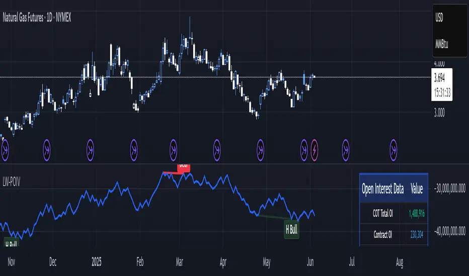
The Larry Williams POIV A/D (Price, Open Interest, Volume Accumulation/Distribution) indicator implements Williams' original formula while adding advanced divergence detection capabilities. This powerful tool combines price movement, open interest, and volume data to identify potential trend reversals and continuations.
FEATURES
--------
- Implements Larry Williams' original POIV A/D formula
- Divergence detection system:
* Regular divergences for trend reversal signals
* Hidden divergences for trend continuation signals
- Fast Mode option for earlier pivot detection
- Customizable sensitivity for divergence filtering
- Dynamic color visualization based on indicator direction
- Adjustable smoothing to reduce noise
- Automatic fallback to OBV when Open Interest is unavailable
FORMULA
-------
POIV A/D = CumulativeSum(Open Interest * (Close - Close ) / (True High - True Low)) + OBV
Where:
- Open Interest: Current period's open interest
- Close - Close : Price change from previous period
- True High - True Low: True Range
- OBV: On Balance Volume
DIVERGENCE TYPES
---------------
1. Regular Divergences (Reversal Signals):
- Bullish: Price makes lower lows while indicator makes higher lows
- Bearish: Price makes higher highs while indicator makes lower highs
2. Hidden Divergences (Continuation Signals):
- Bullish: Price makes higher lows while indicator makes lower lows
- Bearish: Price makes lower highs while indicator makes higher highs
REQUIREMENTS
-----------
- Works best with futures and other instruments that provide Open Interest data
- Automatically adapts to work with any instrument by using OBV when OI is unavailable
USAGE GUIDE
-----------
1. Apply the indicator to any chart
2. Configure settings:
- Adjust sensitivity for divergence detection
- Enable/disable Fast Mode for earlier signals
- Customize visual settings as needed
3. Look for divergence signals:
- Regular divergences for potential trend reversals
- Hidden divergences for trend continuation opportunities
4. Use the alerts system for automated divergence detection
KNOWN LIMITATIONS
----------------
- Requires Open Interest data for full functionality
- Fast Mode may generate more signals but with lower reliability
ACKNOWLEDGEMENTS
---------------
This indicator is based on Larry Williams' work on Open Interest analysis. The implementation includes additional features for divergence detection while maintaining the integrity of the original formula.
Buscar en scripts para "Futures"
HTF Anchored FanSimilar to an Anchored VWAP, this lets you click a bar on an Daily, Weekly, or Monthly chart to add an "Anchored Fan" which displays lines at up to 6 levels above and below the chosen Anchor Point. Useful to measure the retracement during swing moves.
You can reposition the fan by either hovering over the anchor or by clicking the name of the study to "activate" it, and then dragging. You can also change the Anchor Point in Settings.
By default the anchor uses the bar Close, but you can change this manually in settings OR you can use the fancy "Auto high/low" mode which is handy if you are mainly dropping the fan on local swing highs and lows.
The default line measures were chosen for ES (Futures) but the study should be usable with nearly anything as long as you adjust the settings to something appropriate for the ticker. If you want to use this on NQ, for example, it would be reasonable to multiple each of these settings by 3.5 or so.
NOTE: If the fan is way off the left side of the chart it's generally easiest to use Settings to move it back to close to "now".

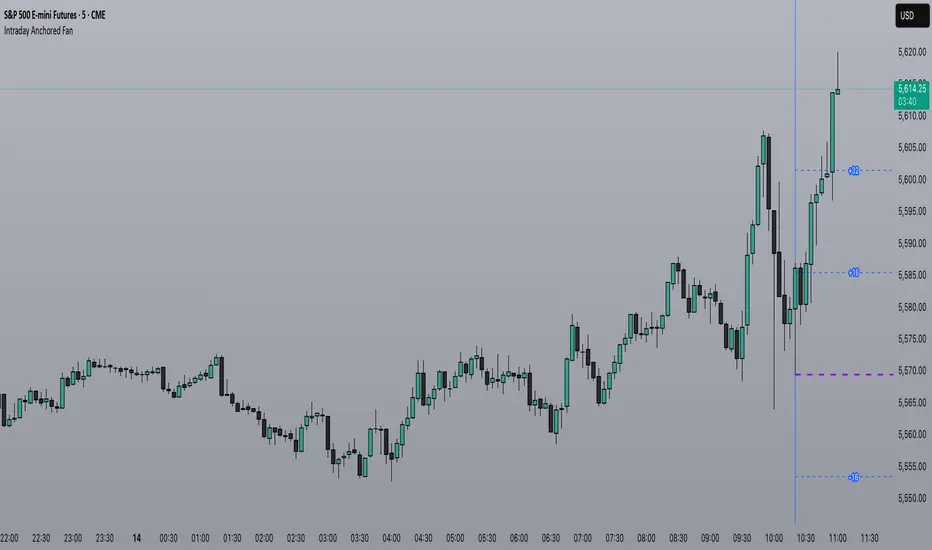
Intraday Anchored FanSimilar to an Anchored VWAP, this lets you click a bar on an Intraday chart to add an "Anchored Fan" which displays lines at up to 6 levels above and below the chosen Anchor Point. Useful to measure the retracement during swing moves.
You can reposition the fan by either hovering over the anchor or by clicking the name of the study to "activate" it, and then dragging. You can also change the Anchor Point in Settings.
By default the anchor uses the bar Close, but you can change this manually in settings OR you can use the fancy "Auto high/low" mode which is handy if you are mainly dropping the fan on local swing highs and lows.
The default line measures were chosen for ES (Futures) but the study should be usable with nearly anything as long as you adjust the settings to something appropriate for the ticker. If you want to use this on NQ, for example, it would be reasonable to multiple each of these settings by 3.5 or so.
NOTE: If the fan is off the left side of the chart, one way to see the Anchor handle again easily is to switch to a higher timeframe; for example if you are on the 5min maybe use the 15min or hourly to find the handle -- if it is WAY off the left side (for example if you let many days pass without advancing it) it's generally easiest to use Settings to move it back to "now".
Lot size calculator for futuresEasily and quickly calculate lot sizes with this unique indicator for futures trading. Whether you're dealing with full contracts or micro contracts, this tool simplifies the process by allowing you to input your account balance, risk percentage, and stop loss in pips. The indicator then automatically calculates the optimal number of contracts to trade based on your risk parameters. Designed for both novice and experienced traders, it ensures precise risk management and enhances your trading strategy. Experience the ease and efficiency of lot size calculation like never before!

Key Times & Opening Prices [Olitrades]This indicator plots key time's (opening prices) with the possibility of vertical separators. It was initially created to utilize on the indices futures market, utilizing ICT logic.
These opening prices are often utilized to determine if price is currently at a premium or a discounted value.
The default times include:
Daily Open (18:00 PM)
Midnight (00:00 AM)
Settlement (15:00 PM)
7:30 AM
8:30 AM
9:30 AM (Equities Open)
10:00 AM (Morning 4h Candle Open)
14:00 PM (Afternoon 4h Candle Open)
Along with up to three custom time slots.
All times used in the indicator are Eastern Standard time (New York local time) and will automatically adjust no matter your time zone.
Historical
When in historical mode, the indicator will keep the previous levels so you can easily visualize them and their relation to price.
You can also choose how many past levels you want to see. This allows you to back test only specific days/weeks.
Other Inputs
The indicator contains an adjustable offset, to modify how far the line extends depending on the current timeframe.
Each one of the above-mentioned levels can be turned on and off, including the custom times. You can also choose between plotting just the opening price, a vertical line separator, or both! All of these lines have adjustable styles (dotted, dashed or solid) and width.
They also have custom cut offs. You may choose specific cut off times for custom time slots (when to stop extending the lines), as well as for AM (before noon) default levels and PM (after noon) default levels.
The indicator also allows to show text labels next to these lines, which is set by default but can be turned off. Custom times also include custom text options.

BB Position CalculatorPosition Size Calculator Instructions
Overview
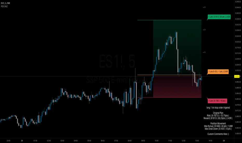
The Position Size Calculator is designed to help traders automatically determine the appropriate lot size based on the dollar amount they are willing to risk. It includes features for automatic lot sizing, fixed lot risk calculations, take profit calculations (both automatic and fixed), max run-up, and max drawdown. Calculated values are displayed in ticks, points, and USD.
Key Features
• Automatic Lot Sizing: Automatically calculates lot size based on the amount of money you are willing to risk.
• Fixed Lot Risk Calculations: Provides risk calculations for fixed lot sizes.
• Take Profit Calculations: Offers both automatic and fixed take profit calculations.
• Max Run-Up and Max Drawdown: Monitors and displays the maximum run-up and drawdown of your trade.
• Detailed Metrics: Displays all calculated values in ticks, points, and USD.
Setup Instructions
1. Add and Remove for Each Position: The calculator is designed to be added to your chart for each new position. Once your preferences are set the first time, save them as your default to retain your settings for future use.
2. Adding the Indicator to Favorites:
• Use the TradingView keyboard shortcut “/” then type “pos.”
• Use the arrow key to select the Position Size Calculator and press enter.
• Close the indicator selection pop-up.
3. Setting the Trigger Price:
• A blue pop-up labeled “SET TRIGGER PRICE” will appear at the bottom of the chart.
• Click on the chart at the price level where you want to enter the trade.
4. Setting the Stop Loss:
• The pop-up will change to “SET STOP LOSS.”
• Click on the chart at the price level where your stop loss will be set.
5. Setting the Take Profit:
• The pop-up will change to “SET TAKE PROFIT.”
• Click on the chart at the price level where you want to take profit. If you have selected the option to overwrite with a set risk/reward ratio (R:R), the calculation will use this price level.
6. Setting the Trade Window Start:
• The pop-up will change to “SET TRADE WINDOW START.”
• Click on the bar in time where you want the indicator to start monitoring for price to trigger the position.
7. Adjusting the Position:
• Clicking on any part of the indicator will display draggable lines, allowing you to fine-tune the position that was previously plotted by the first four chart clicks.
Additional Notes
• Compatibility: This calculator has only been tested with futures trading.
• Customization: Once your preferences are set, save them as your default to make setup quicker for future trades.
• Support: If you have any questions or feature requests, please feel free to reach out.
Captain Backtest Model [TFO]Created by @imjesstwoone and @mickey1984, this trade model attempts to capture the expansion from the 10:00-14:00 EST 4h candle using just 3 simple steps. All of the information presented in this description has been outlined by its creators, all I did was translate it to Pine Script. All core settings of the trade model may be edited so that users can test several variations, however this description will cover its default, intended behavior using NQ 5m as an example.
Step 1 is to identify our Price Range. In this case, we are concerned with the highest high and the lowest low created from 6:00-10:00 EST.
Step 2 is to wait for either the high or low of said range to be taken out. Whichever side gets taken first determines the long/short bias for the remainder of the Trade Window (i.e. if price takes the range high, bias is long, and vice versa). Bias must be determined by 11:15 EST, otherwise no trades will be taken. This filter is intended to weed out "choppy" trading days.
Step 3 is to wait for a retracement and enter with a close through the previous candle's high (if long biased) or low (if short biased). There are a couple toggleable criteria that we use to define a retracement; one is checking for opposite close candles that indicate a pullback; another is checking if price took the previous candle's low (if long biased) or high (if short biased).
This trade model was initially tested for index futures, particularly ES and NQ, using a 5m chart, however this indicator allows us to backtest any symbol on any timeframe. Creators @imjesstwoone and @mickey1984 specified a 5 point stop loss on ES and a 25 point stop loss on NQ with their testing.
I've personally found some success in backtesting NQ 5m using a 25 point stop loss and 75 point profit target (3:1 R). Enabling the Use Fixed R:R parameter will ensure that these stops and targets are utilized, otherwise it will enter and hold the position until the close of the Trade Window.

Show Extended Hours (Futures & Crypto)OVERVIEW
This indicator mimics TradingViews "Extended trading hours" background color settings. It is most useful on symbols that do not conventionally have extended hours, but are available to trade during those hours (ie. Futures and Crypto). Because market participation (ie. volatility) in a given symbol can change dramatically at or near these transitions, seeing conventional market open / closures expedites price action context around these transitions.
INPUTS
You can configure:
Background colors for both Premarket and After Hours
Which extended hours you would like to see
Market Hours and Time Zone

Pin Candle DetectionPin candles are a variation of hammer candles that are useful in technical analysis . In particular, when combined with volume profile studies, they can be a powerful set up for long entries or other decision making.
For example, when looking at volume profiles, a long entry would be a fair value area (i.e. 40%) below the close of a pin candle. When combined with a support level , the set up is stronger.
While most scripts look for hammer candles, pin candles are somewhat different in that the length of the wick is significant.
This script and its parameters was built for ES futures 15 min chart in mind.
This script is unique in that it allows for the below parameters to be adjusted to suit other instruments and timeframes:
1. Fib level: Candle must close within a certain retracement level). My preference is 0.55. Some traders like 0.5, while others prefer 0.33
2. Wick length: Pin candles differ from pure hammers in that the length of the wick must be significant. My preference is 7 points on ES (as in $ and not ticks)
Add this script to your alerts to no longer miss these set ups.

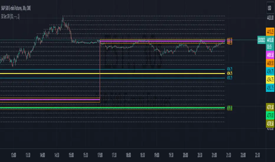
30 Second Futures Session Open RangeThis indicator displays 30 second opening ranges from Globex, Europe, and RTH sessions.
From the RTH session range, it also displays infinitely generating Price Targets based on a % of the opening range size.
I am retrieving the 30 second data using the new "request.security_lower_tf()" function.
The importance of these levels is based on the idea that when the market opens, algorithms establish their positions within the first 30 seconds.
These areas can also be seen as potential areas of support and resistance throughout the sessions.
Enjoy!
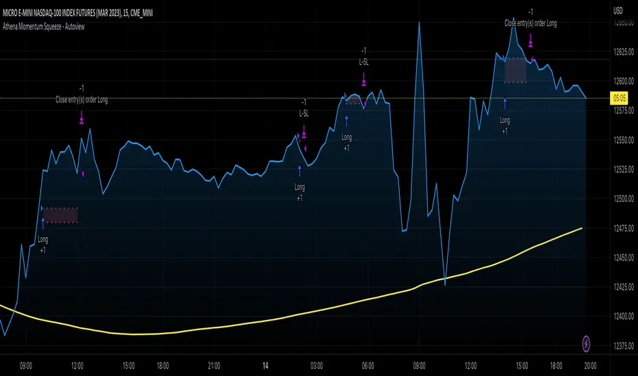
Athena Momentum Squeeze - Short, Lean, and Mean This is a very profitable strategy focusing on 15 minute intervals on the Micro Nasdaq Futures contracts. CME_MINI:MNQH2023
As this contract only keeps positions for on average about an hour risk is managed. At a profit factor of 3.382 with a max drawdown of $123 from January 1st to February 15. Looking back to Dec 2019 still maintains a profit factor of 1.3.
See backtesting: www.screencast.com
2019 backtesting: www.screencast.com
Based on the classic Lazy Bear Oscillator Squeeze with a number of modifications from ADX, MAs and adding fibonacci levels.
We like keeping strategies simple yet powerful, no completely where you can't understand your own trades.
Our team is always modifying and improving the strategy. Always open to collaborating on improving as there is no perfect strategy. www.screencast.com
Historical Federal Fund Futures CurveUse this indicator to plot the federal funds futures implied rates term structure against historical curves
Based upon the work of @BarefootJoey, @longfiat, @OpptionsOnly

Session LiquidityThe “Session Liquidity” TradingView indicator by Infinity Trading creates dynamic horizontal lines at the high and low points of a specified time span within the trading day. This indicator gives the user control of three separate time spans so the user can dynamically see the highs and lows of their favorite daily time spans.
Purpose
This indicator is similar to my TradingView indicator “Futures Exchange Sessions 3.0”. In that indicator the user gets control of dynamic price boxes. For me, these boxes made it difficult to spot ICT’s Orderblocks. So instead of boxes I made independently controllable lines and now I can spot ICT Orderblocks and easily identify Liquidity Pools.
Inputs and Style
Everything about the three dynamic lines can but independently configured. Start & End Times, Line Color, Line Style, Line Width, Text Characters, Text Size, Text Color can all be adjusted. The high and low lines as well as their text labels can be individually toggled on or off for maximum control.
Timezone
All of the start and end times are in EST. Additionally, each time span line needs a specific start of each day. This is controlled by a setting called “Line Start Day Timezone” where the user sets a timezone that corresponds with the start time. In general if a timespan resides within a particular Session pick the corresponding timezone. If the users line fits in the Asian Session then choose Asia/Shanghai. If the line is within the London Session then choose Europe/London. And the same goes for the New York Session.
Special Notes
If the Line Start Time is within one candle of the Start Day Timezone in the Settings, then the line/box won’t display. So choose the previous timezone
Lines only display when the timeframe is <= 30 minute
Gallery

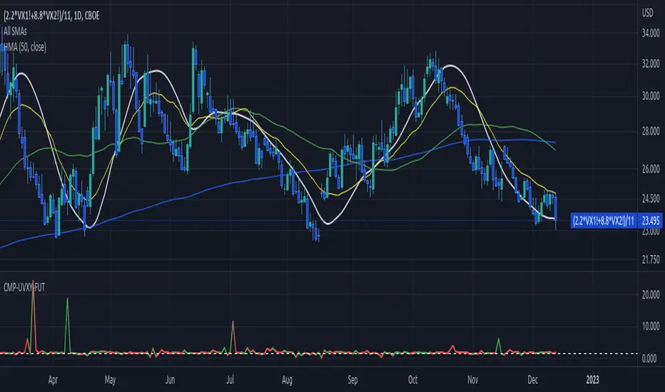
Compare UVXY to its VIX futures basketJust a quick script to show the actual movement ration between UVXY and its VIX futures basket.
The advertised reference value of 1.5 is shown as well.
The basket is hardcoded for now. Depending on how the underlyings of UVXY change, this might have to be configurable.
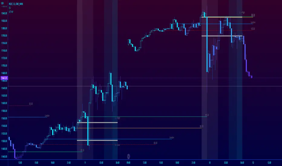
ICT NY Futures Indices Session Model - YT New York MentorshipThis indicator plots out the time periods and open lines as outlined in ICT's 2022 Mentorship and is designed specifically for the New York futures trading session.
Time zone is set to GMT-4 (NY) by default but can be changed for accommodate daylight saving in the menu.
Please note this indicator is to be used only on the 30min timeframe and below.
Here are its features:
The background color shows the morning session, in two parts (8.30am to 9.30am and 9.30am to 11.30am), then a two hour gap for lunch (ICT calls this "Dead time") and finally, the afternoon session, also to two (1.30pm to 3pm and 3pm to 4pm).
It not only shows the current killzones, but future zones as well.
These times are important; trades can be framed within these zones as taught in the mentorship.
Next are the open lines. These lines are automatically plotted and can be areas for price to react off of; they are the opening price of a candle at these times:
00.00 (New York Midnight, also known as "True Day Open")
8.30am (New York Equities pre-open)
9.30am (New York Equities open)
2.00am (London Stock Exchange open)
And lastly, London's trading session High and Low are projected forward onto the New York trading session.
These two price points are areas of liquidity that were pooled during London, but they can also often set the high or low of the day.
Please let me know if there are any bugs or if you have suggestions for the next update.
Crypto BTC Correlation Scalper Gaps StrategyThis strategy is based on the gaps theory.
In this case we have the BTC futures from CME, which acts in a way similar to stocks, and we can have gaps present between close/open session, and also sometimes between same candle due to huge movements intra candle.
At the same time I have combined this with a daily moving average, to help out a bit with the trend, since we are looking at small timeframe like 1-15/30min .
On top of that we have a reverse option, where long = short and viceversa, which can be used with against BTC pairs .
Rule are simple:
For long, we have a long gap and the close of the correlated candle is above daily sma
For short, we have a short gap and the close of the correlated candle is below daily sma
For exit:
For exit, we take the highest highest values for short entry TP, meaning we get the different from the HH and rest the current open candle distance, and use that distance as a TP.
At the same time for long entry, we take the lowest low value and rest current close of the candle to that value, and we get the TP.
Can also be applied this logic for SL aswell but from the test I have found out that exiting based on a reverse condition(when tp is not being hit), gives better results/dd overall.
If you have any questions, please let me know !

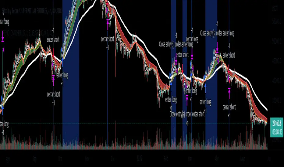
EMA_TREND_CATCHERSimple strategy based on the crossing of moving averages of 50,100 and 200 periods. Designed to identify trends
You are ready to use trading bots (all you have to do is fill in "Variables for Alert"). However, it can also be used for discretionary operations.
BTCUSDT FUTURES BINANCE
4H
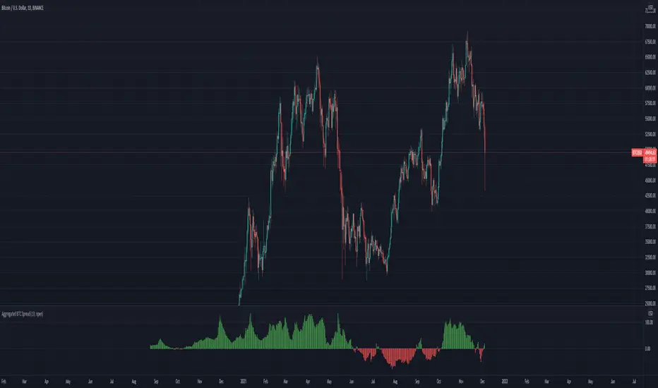
BTC Spot/Futures Volume RatioShows the ratio between the spot trading volume versus futures trading volume for Bitcoin. This ratio may be interpreted as how active the market currently is, and may lead to various interpretations. For example, when the price is at a high level and this ratio gradually decreases, it may imply the end of the distribution phase; when the price is low and the ratio is at the bottom, it may imply the bottom of the price.

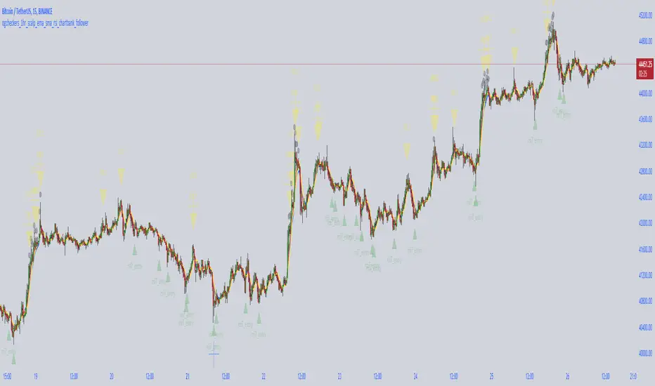
crypto futures hourly scalping with ma & rsi - ogcheckershi to all lovable traders,
hereby i want to share a combination of trade ideas for scalping
i've chosen hourly timeframe
indicators used: moving averages and rsi
moving averages:
ema 3, ema 5, ema 7
sma 3, sma 5, sma 7
daily_ema_3, daily_ema_5
daily_ema_5, daily_sma_5
rsi:
rsi 7, rsi 14, rsi 26
daily_rsi_7, daily_rsi_14, daily_rsi_26
as per the analysis over moving average behavioral patterns & rsi movements, useful points are given below which will be helpful while choosing good entry points & exit points,
strategical points for LONG:
* when ema3 crosses above sma3 - green candles start to form
* it's followed by ema5 > sma5 and ema7 > sma7
* when ema3 crosses down sma3 - it's considered as an indication of exit
* if rsi supports then can wait for ema5 crossing down sma5
* as similar, when daily_ema_3 crosses above daily_sma_3, its an higher timeframe bullish indication, so the lower timeframe entries inside this higher timeframe is a sure shot confident entry
* for LONG always take entries when rsi_14 < 30 or 25 else check rsi_7 < 25 or below
* as along the above, bullish CANDLE patterns like bullish engulfing , morning star is been used for entry at lower levels
* so here i've used OPEN as rsi_source in majority
* exit points also indicated at high_rsi and moving average crossunders or reverse crossovers
* for SHORTING, the above said ideas can be used in viceversa
* inputs in the indicator were tailored for users needs so that you will enjoy the magics of customization
if i am wrong in anyways regarding the above indicator strategy, please forgive me and help me improve in this aspect by commenting.
after few more studies and analysis and mainly QUERIES & COMMENTS, i'm planning to backtest these strategies here in tradingview.
also if these strategies are coded in python, we can link it to Binance Futures Algo or Bot Trading.
thankyou for this opportunity,
thanks to tradingview and pinecoders
thanks to Pranab (for 365MA)
thanks to Gandalf (for inspiring)
Special Thanks & Love to Chartbank for Everything
Bubbles BB futuresQuick and simple BB bubble indicator for Futures
Draw an arrow if candle corpse is out of Bollinger Band (Upper / Lower)
It's not a signal.
I use it to off-load my charts

Dynamic Momentum Ecosystem Futures verI've reuploaded my previous uploaded script Dynamic Momentum Ecosystem, but this one specifically catered to futures trading.
The idea and underlying script function as usual.
Lime = Price closed higher + volume transacted higher than average + MACD Histogram increases + 13 EMA increases
Green = Price closed higher + MACD Histogram increases + 13 EMA increases
Red = Price closed lower + MACD Histogram decreases + 13 EMA decreases
Blue = Either MACD Histogram increases/decreases + 13 EMA increases/decreases
Lime candle is viewed as a robust bullish sign as price increases, supported by the rising MACD Histogram, 13EMA, and higher than average volumes transacted. Perfect for dip buying near the 20/50 MAs.
Green candle is viewed as bullish with the rising of MACD Histogram and EMA . Good for dip buying near the 20/50 MAs.
Red candle is viewed as bearish with the declining of MACD Histogram and EMA . Good for short entry. Can also be the early sign to take profits, as it could be the preliminary signal for trend reversal.
Blue candle is viewed as neutral.
The upper dotted purple line is the 52candles high.
The vertical grey line appears when the price > MA50 crosses above MA200, which is a golden crossover.
Traders are advised to time their entry using the impulse coloring system for stocks that are trading near the dotted line, following the grey line formation.

[GB]Commodity Futures MapPuts numerous commodity futures on the same scale. The main function is RSI (without evoking "oversold/bought" concepts).
Reading the chart: Much like any oscillator, the important elements are:
Position relative to the middle
Slope
Momentum
Volatility
Settings:
RSI length
EMA smoothing
Time Frame (of the indicator, not the chart(
May add value when asking questions like:
Is lumber trending?
Is silver trending faster than gold?
Is the entire asset class trending up down or not at all?
Adding additional symbols is easy since the code for each symbol is identical.

Aggregated BTC SpreadThis script is used to aggregate the bitcoin spread on futures contracts on different platforms.
It works by averaging the for every selected exchange, and apply an EMA of .
It is supporting
Binance (USD / USDT)
Okex
FTX
Huobi
Deribit
Ascendex
CME (BTC1!)