Buscar en scripts para "Buy sell"
ZenTrend Follower Signals (Backtest)Buy/Sell Entry signals based on the ZenTrend Follower indicator.
Entries are taken from the setup and trend breakout level, exits from the trailing stop loss.
Overextension and trend re-entry signals are ignored.
The indicator is linked below
If you enjoy these posts please like and subscribe so more people can join you :)
If you want to tryout the indicator and strategy, follow me and drop a comment or pm and I’ll get you set up.
Stay calm, and happy trading!
More information on the indicator can be found below:

Altcoins StrategyBuy/Sell Altcoins strategy. Based on moving averages, divergences, price and volume

Buy SellKıvanc hocanın yazdığı 2 stop loss indikatörünün birleşmesi sonucu bulundu. Çalışma mantığını kullandıkça anlayacaksınızıdır.


Buy Sell signal by Spicytrader
Get on board before going to the moon !
Spicytrader instantly identifies when a potential pump or dump is beginning.
Compatible with Autoview bot
GET ACCESS : spicytrader.com


Buy/Sell Using MACD and ReversalsUsing the crossover of Signal Line and MACD line predict the reversals of trends in the chart.


Buy/Sell Ahmed Rashiedtrade with confidence good for both intra day and long term took me 2 yrs to finish it

MULTIPLE TIME-FRAME STRATEGY(TREND, MOMENTUM, ENTRY) Hey everyone, this is one strategy that I have found profitable over time. It is a multiple time frame strategy that utilizes 3 time-frames. Highest time-frame is the trend, medium time-frame is the momentum and short time-frame is the entry point.
Long Term:
- If closed candle is above entry then we are looking for longs, otherwise we are looking for shorts
Medium Term:
- If Stoch SmoothK is above or below SmoothK and the momentum matches long term trend then we look for entries.
Short Term:
- If a moving average crossover(long)/crossunder(short) occurs then place a trade in the direction of the trend.
Close Trade:
- Trade is closed when the Medium term SmoothK Crosses under/above SmoothD.
You can mess with the settings to get the best Profit Factor / Percent Profit that matches your plan.
Best of luck!
[STRATEGY][RS]MicuRobert EMA cross V2Great thanks Ricardo , watch this man . Start at 2014 December with 1000 euro.


Pivot Breakout + EMA Stack + Vol + Candle ConfirmThis indicator combines pivot breakout logic with trend, volume, and price action confirmations to filter strong trading opportunities.
🔹 Key Features:
Dynamic Pivot Levels (Fibonacci, Traditional, Camarilla, Woodie, etc.) across multiple timeframes (Daily → Yearly).
EMA Stack Trend Filter (20/50/100/200 EMA alignment for bullish/bearish confirmation).
Volume Confirmation (breakouts validated by volume > SMA).
Candle Body Strength Filter (optional strict mode: candle body ≥ % of range).
Breakout Signals (BUY when price breaks above pivot resistances in bullish trend; SELL when breaking below supports in bearish trend).
Consolidation Zone Highlight (between R1 & S1).
Visual Alerts & Signals (BUY/SELL markers + TradingView alertcondition).
✅ Works across all assets (stocks, crypto, forex, futures).
✅ Ideal for breakout traders, trend-followers, and swing traders.
✅ Customizable pivots, EMAs, volume filter, and candle confirmation for flexible strategies.
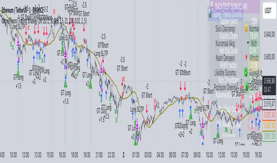
Game Theory Trading StrategyGame Theory Trading Strategy: Explanation and Working Logic
This Pine Script (version 5) code implements a trading strategy named "Game Theory Trading Strategy" in TradingView. Unlike the previous indicator, this is a full-fledged strategy with automated entry/exit rules, risk management, and backtesting capabilities. It uses Game Theory principles to analyze market behavior, focusing on herd behavior, institutional flows, liquidity traps, and Nash equilibrium to generate buy (long) and sell (short) signals. Below, I'll explain the strategy's purpose, working logic, key components, and usage tips in detail.
1. General Description
Purpose: The strategy identifies high-probability trading opportunities by combining Game Theory concepts (herd behavior, contrarian signals, Nash equilibrium) with technical analysis (RSI, volume, momentum). It aims to exploit market inefficiencies caused by retail herd behavior, institutional flows, and liquidity traps. The strategy is designed for automated trading with defined risk management (stop-loss/take-profit) and position sizing based on market conditions.
Key Features:
Herd Behavior Detection: Identifies retail panic buying/selling using RSI and volume spikes.
Liquidity Traps: Detects stop-loss hunting zones where price breaks recent highs/lows but reverses.
Institutional Flow Analysis: Tracks high-volume institutional activity via Accumulation/Distribution and volume spikes.
Nash Equilibrium: Uses statistical price bands to assess whether the market is in equilibrium or deviated (overbought/oversold).
Risk Management: Configurable stop-loss (SL) and take-profit (TP) percentages, dynamic position sizing based on Game Theory (minimax principle).
Visualization: Displays Nash bands, signals, background colors, and two tables (Game Theory status and backtest results).
Backtesting: Tracks performance metrics like win rate, profit factor, max drawdown, and Sharpe ratio.
Strategy Settings:
Initial capital: $10,000.
Pyramiding: Up to 3 positions.
Position size: 10% of equity (default_qty_value=10).
Configurable inputs for RSI, volume, liquidity, institutional flow, Nash equilibrium, and risk management.
Warning: This is a strategy, not just an indicator. It executes trades automatically in TradingView's Strategy Tester. Always backtest thoroughly and use proper risk management before live trading.
2. Working Logic (Step by Step)
The strategy processes each bar (candle) to generate signals, manage positions, and update performance metrics. Here's how it works:
a. Input Parameters
The inputs are grouped for clarity:
Herd Behavior (🐑):
RSI Period (14): For overbought/oversold detection.
Volume MA Period (20): To calculate average volume for spike detection.
Herd Threshold (2.0): Volume multiplier for detecting herd activity.
Liquidity Analysis (💧):
Liquidity Lookback (50): Bars to check for recent highs/lows.
Liquidity Sensitivity (1.5): Volume multiplier for trap detection.
Institutional Flow (🏦):
Institutional Volume Multiplier (2.5): For detecting large volume spikes.
Institutional MA Period (21): For Accumulation/Distribution smoothing.
Nash Equilibrium (⚖️):
Nash Period (100): For calculating price mean and standard deviation.
Nash Deviation (0.02): Multiplier for equilibrium bands.
Risk Management (🛡️):
Use Stop-Loss (true): Enables SL at 2% below/above entry price.
Use Take-Profit (true): Enables TP at 5% above/below entry price.
b. Herd Behavior Detection
RSI (14): Checks for extreme conditions:
Overbought: RSI > 70 (potential herd buying).
Oversold: RSI < 30 (potential herd selling).
Volume Spike: Volume > SMA(20) x 2.0 (herd_threshold).
Momentum: Price change over 10 bars (close - close ) compared to its SMA(20).
Herd Signals:
Herd Buying: RSI > 70 + volume spike + positive momentum = Retail buying frenzy (red background).
Herd Selling: RSI < 30 + volume spike + negative momentum = Retail selling panic (green background).
c. Liquidity Trap Detection
Recent Highs/Lows: Calculated over 50 bars (liquidity_lookback).
Psychological Levels: Nearest round numbers (e.g., $100, $110) as potential stop-loss zones.
Trap Conditions:
Up Trap: Price breaks recent high, closes below it, with a volume spike (volume > SMA x 1.5).
Down Trap: Price breaks recent low, closes above it, with a volume spike.
Visualization: Traps are marked with small red/green crosses above/below bars.
d. Institutional Flow Analysis
Volume Check: Volume > SMA(20) x 2.5 (inst_volume_mult) = Institutional activity.
Accumulation/Distribution (AD):
Formula: ((close - low) - (high - close)) / (high - low) * volume, cumulated over time.
Smoothed with SMA(21) (inst_ma_length).
Accumulation: AD > MA + high volume = Institutions buying.
Distribution: AD < MA + high volume = Institutions selling.
Smart Money Index: (close - open) / (high - low) * volume, smoothed with SMA(20). Positive = Smart money buying.
e. Nash Equilibrium
Calculation:
Price mean: SMA(100) (nash_period).
Standard deviation: stdev(100).
Upper Nash: Mean + StdDev x 0.02 (nash_deviation).
Lower Nash: Mean - StdDev x 0.02.
Conditions:
Near Equilibrium: Price between upper and lower Nash bands (stable market).
Above Nash: Price > upper band (overbought, sell potential).
Below Nash: Price < lower band (oversold, buy potential).
Visualization: Orange line (mean), red/green lines (upper/lower bands).
f. Game Theory Signals
The strategy generates three types of signals, combined into long/short triggers:
Contrarian Signals:
Buy: Herd selling + (accumulation or down trap) = Go against retail panic.
Sell: Herd buying + (distribution or up trap).
Momentum Signals:
Buy: Below Nash + positive smart money + no herd buying.
Sell: Above Nash + negative smart money + no herd selling.
Nash Reversion Signals:
Buy: Below Nash + rising close (close > close ) + volume > MA.
Sell: Above Nash + falling close + volume > MA.
Final Signals:
Long Signal: Contrarian buy OR momentum buy OR Nash reversion buy.
Short Signal: Contrarian sell OR momentum sell OR Nash reversion sell.
g. Position Management
Position Sizing (Minimax Principle):
Default: 1.0 (10% of equity).
In Nash equilibrium: Reduced to 0.5 (conservative).
During institutional volume: Increased to 1.5 (aggressive).
Entries:
Long: If long_signal is true and no existing long position (strategy.position_size <= 0).
Short: If short_signal is true and no existing short position (strategy.position_size >= 0).
Exits:
Stop-Loss: If use_sl=true, set at 2% below/above entry price.
Take-Profit: If use_tp=true, set at 5% above/below entry price.
Pyramiding: Up to 3 concurrent positions allowed.
h. Visualization
Nash Bands: Orange (mean), red (upper), green (lower).
Background Colors:
Herd buying: Red (90% transparency).
Herd selling: Green.
Institutional volume: Blue.
Signals:
Contrarian buy/sell: Green/red triangles below/above bars.
Liquidity traps: Red/green crosses above/below bars.
Tables:
Game Theory Table (Top-Right):
Herd Behavior: Buying frenzy, selling panic, or normal.
Institutional Flow: Accumulation, distribution, or neutral.
Nash Equilibrium: In equilibrium, above, or below.
Liquidity Status: Trap detected or safe.
Position Suggestion: Long (green), Short (red), or Wait (gray).
Backtest Table (Bottom-Right):
Total Trades: Number of closed trades.
Win Rate: Percentage of winning trades.
Net Profit/Loss: In USD, colored green/red.
Profit Factor: Gross profit / gross loss.
Max Drawdown: Peak-to-trough equity drop (%).
Win/Loss Trades: Number of winning/losing trades.
Risk/Reward Ratio: Simplified Sharpe ratio (returns / drawdown).
Avg Win/Loss Ratio: Average win per trade / average loss per trade.
Last Update: Current time.
i. Backtesting Metrics
Tracks:
Total trades, winning/losing trades.
Win rate (%).
Net profit ($).
Profit factor (gross profit / gross loss).
Max drawdown (%).
Simplified Sharpe ratio (returns / drawdown).
Average win/loss ratio.
Updates metrics on each closed trade.
Displays a label on the last bar with backtest period, total trades, win rate, and net profit.
j. Alerts
No explicit alertconditions defined, but you can add them for long_signal and short_signal (e.g., alertcondition(long_signal, "GT Long Entry", "Long Signal Detected!")).
Use TradingView's alert system with Strategy Tester outputs.
3. Usage Tips
Timeframe: Best for H1-D1 timeframes. Shorter frames (M1-M15) may produce noisy signals.
Settings:
Risk Management: Adjust sl_percent (e.g., 1% for volatile markets) and tp_percent (e.g., 3% for scalping).
Herd Threshold: Increase to 2.5 for stricter herd detection in choppy markets.
Liquidity Lookback: Reduce to 20 for faster markets (e.g., crypto).
Nash Period: Increase to 200 for longer-term analysis.
Backtesting:
Use TradingView's Strategy Tester to evaluate performance.
Check win rate (>50%), profit factor (>1.5), and max drawdown (<20%) for viability.
Test on different assets/timeframes to ensure robustness.
Live Trading:
Start with a demo account.
Combine with other indicators (e.g., EMAs, support/resistance) for confirmation.
Monitor liquidity traps and institutional flow for context.
Risk Management:
Always use SL/TP to limit losses.
Adjust position_size for risk tolerance (e.g., 5% of equity for conservative trading).
Avoid over-leveraging (pyramiding=3 can amplify risk).
Troubleshooting:
If no trades are executed, check signal conditions (e.g., lower herd_threshold or liquidity_sensitivity).
Ensure sufficient historical data for Nash and liquidity calculations.
If tables overlap, adjust position.top_right/bottom_right coordinates.
4. Key Differences from the Previous Indicator
Indicator vs. Strategy: The previous code was an indicator (VP + Game Theory Integrated Strategy) focused on visualization and alerts. This is a strategy with automated entries/exits and backtesting.
Volume Profile: Absent in this strategy, making it lighter but less focused on high-volume zones.
Wick Analysis: Not included here, unlike the previous indicator's heavy reliance on wick patterns.
Backtesting: This strategy includes detailed performance metrics and a backtest table, absent in the indicator.
Simpler Signals: Focuses on Game Theory signals (contrarian, momentum, Nash reversion) without the "Power/Ultra Power" hierarchy.
Risk Management: Explicit SL/TP and dynamic position sizing, not present in the indicator.
5. Conclusion
The "Game Theory Trading Strategy" is a sophisticated system leveraging herd behavior, institutional flows, liquidity traps, and Nash equilibrium to trade market inefficiencies. It’s designed for traders who understand Game Theory principles and want automated execution with robust risk management. However, it requires thorough backtesting and parameter optimization for specific markets (e.g., forex, crypto, stocks). The backtest table and visual aids make it easy to monitor performance, but always combine with other analysis tools and proper capital management.
If you need help with backtesting, adding alerts, or optimizing parameters, let me know!
Volume Comparison with Buyer/Seller PressureTHIS indicator is well-structured and provides a comprehensive way to analyze volume alongside buyer and seller pressure. This indicator helps traders analyze volume dynamics in the stock or cryptocurrency market while simultaneously assessing buyer and seller pressure. Its use case revolves around identifying strong buying or selling activity, neutral conditions, and volume trends over different time periods. Below is a breakdown of how to use this indicator:
This Pine Script indicator helps traders analyze volume dynamics in the stock or cryptocurrency market while simultaneously assessing buyer and seller pressure. Its use case revolves around identifying strong buying or selling activity, neutral conditions, and volume trends over different time periods. Below is a breakdown of how to use this indicator:
Key Features and Use Case
Volume-Based Insights:
Displays daily volume and compares it to the 3-day, 5-day, 10-day, and 20-day moving averages of volume. Helps traders identify days with unusual volume spikes relative to historical averages, signaling potential reversals or breakouts.
Buyer and Seller Pressure:
Measures buyer pressure: how much the closing price dominates the trading range of the day.
Measures seller pressure: how much the opening price dominates the trading range of the day.
Highlights areas where buying or selling pressure is particularly strong (≥ 0.75).
Background Signals:
Green Background: Strong buyer pressure (indicative of potential upward momentum).
Red Background: Strong seller pressure (indicative of potential downward momentum).
Gray Background: Neutral market conditions (neither buying nor selling dominance).
Alerts:
Alerts traders when:
Strong buying signals are detected.
Strong selling signals are detected.
The market is neutral, with neither buyers nor sellers in control.
Decision-Making Aid:
Combines volume analysis with price action (buyer/seller pressure) to help traders identify:
Potential breakout opportunities.
Reversal points.
Neutral zones where a trader might avoid trading due to indecision in the market.
How to Use It in Trading:------->
Add the Indicator:
Apply this Indicator to your Trading View chart to start visualizing the buyer/seller pressure and volume averages.
Interpret Volume Trends:
Look for days when daily volume significantly exceeds the 3-day, 5-day, 10-day, or 20-day average.
These could indicate:
A breakout when aligned with strong buyer pressure.
A sell-off when aligned with strong seller pressure.
React to Background Colors:
* Green Background (Strong Buyer Pressure):
Suggests buyers are dominating the market, and upward momentum is likely.
Use this signal to consider buying opportunities, especially if volume is above average.
* Red Background (Strong Seller Pressure):
Indicates sellers are in control, and prices might fall.
Use this signal to consider selling or shorting opportunities.
* Gray Background (Neutral Market):
Reflects indecision; avoid entering trades during these periods unless other signals support a strategy.
Volume Confirmation:
Combine volume analysis with buyer/seller pressure to confirm trends.
Example: A high daily volume with strong buyer pressure signals a high-probability uptrend.
Set Alerts:
Enable alerts to receive real-time notifications when the market generates strong buy/sell signals or enters a neutral zone.
Who Can Benefit:
* Day Traders: Quickly assess intraday market dynamics and volume trends.
* Swing Traders: Identify breakout opportunities or reversal points based on strong buyer/seller pressure.
* Volume Analysts: Compare historical volume averages to current conditions for deeper insights.
Limitations:
Does not guarantee success—should be combined with other technical indicators or strategies.
In low-volume markets, signals may produce false positives or unreliable results.
Assumes traders have basic knowledge of price action and volume analysis.
By integrating this indicator into your strategy, you gain a powerful tool to analyze buyer/seller dominance alongside volume trends, improving your market timing and trade execution.
The Buyer and Seller Pressure components in this indicator provide crucial insights into the market's sentiment and momentum by analyzing the price action relative to the trading volume. Here's how they are used:
1. Buyer Pressure:
Formula:
Buyer Pressure = (Close − Open) / (High − Low )
Interpretation:
* A high buyer pressure (≥ 0.75) indicates strong bullish sentiment, where the price closes much higher than it opened, and the range (high-low) is sufficiently wide.
* It identifies periods of aggressive buying, often signaling potential bullish trends or confirming upward momentum.
2. Seller Pressure:
Formula:
Seller Pressure = (Close − Open ) / (High -Low )
Interpretation:
*A high seller pressure (≥ 0.75) suggests strong bearish sentiment, where the price closes much lower than it opened, within a wide range.
*It helps identify periods of aggressive selling, signaling potential bearish trends or downward momentum.
Purpose in the Indicator:
1. Market Sentiment Analysis:
* Buyer Pressure and Seller Pressure allow traders to gauge market sentiment—whether buyers or sellers dominate a particular time frame.
* This helps in identifying trend reversals or confirmations.
2. Decision-Making Framework:
* The indicator uses thresholds (default 0.75) to classify the market into:
* Strong Buy Signal: When buyer pressure is dominant.
* Strong Sell Signal: When seller pressure is dominant.
* Neutral Signal: When neither buyer nor seller pressure dominates.
*This classification provides a straightforward decision-making tool for traders.
Risk Management:
*By identifying periods of strong buying or selling, traders can avoid entering trades in highly volatile or one-sided markets, which helps reduce risk.
Volume Confirmation:
*Integrating volume data with buyer/seller pressure helps confirm trends. For example:
*High buyer pressure accompanied by higher-than-average volume strengthens the bullish signal.
*Similarly, high seller pressure with higher-than-average volume confirms bearish signals.
Trade Timing:
*The indicator highlights conditions of potential entry (strong buy) or exit (strong sell), allowing traders to time their trades better based on real-time market activity.
Use Case:
*Example:
*Suppose the indicator shows Buyer Pressure = 0.85 with daily volume above the 3-day average. This combination suggests strong bullish activity with momentum, signaling a buy opportunity.
*Conversely, if Seller Pressure = 0.80 with volume above the 5-day average, it signals strong bearish momentum, ideal for selling or shorting.
This indicator combines buyer/seller pressure with volume dynamics, making it valuable for short-term and intraday traders looking for precise market entries and exits.
The background color in this indicator plays an important visual role in helping traders quickly identify the market sentiment based on buyer and seller pressure. It provides a dynamic, color-coded background that changes depending on the strength of the market's buying or selling activity.
Here's how it works:
Background Color Logic:
1. Green Background (Strong Buy Signal):
*Condition: The background turns green when buyer pressure is greater than or equal to 0.75 (strong buying pressure).
*Interpretation: A green background indicates that there is significant bullish sentiment in the market, with strong buying activity. Traders can interpret this as an environment conducive to buying or holding long positions.
*Visual Effect: This helps to quickly spot bullish market conditions, reinforcing potential entry signals for buyers.
2.Red Background (Strong Sell Signal):
*Condition: The background turns red when seller pressure is greater than or equal to 0.75 (strong selling pressure).
*Interpretation: A red background indicates that the market is dominated by selling, showing strong bearish sentiment. Traders can consider this as a signal to sell or short the asset.
*Visual Effect: The red background highlights moments when the market is heavily selling, prompting traders to either exit long positions or take short positions.
Gray Background (Neutral/Indecision Zone):
Condition: The background turns gray when neither buyer nor seller pressure exceeds 0.75. This means the market is neutral, with no dominant bullish or bearish sentiment.
Interpretation: A gray background suggests market indecision or balance between buyers and sellers. It can indicate periods of consolidation or sideways movement where no strong trend is forming.
Visual Effect: The gray background helps traders avoid entering trades when the market lacks a clear direction or when the sentiment is neutral, reducing risk during indecisive times.
Practical Use:
Instant Visual Confirmation:
*Traders can use the background color as an instant confirmation of the market’s sentiment. For instance, if the background turns green, traders might feel more confident in making a long (buy) trade.
*If the background turns red, it serves as a strong visual cue to short or exit a long position.
Helps with Trade Timing:
*The background color can be used in conjunction with other indicators and volume data to time entries and exits more effectively. For example:
*A green background with strong volume indicates a strong trend that could justify a buy.
*A red background with a significant volume surge signals strong selling pressure, which could prompt a sell.
Simplifies Market Analysis:
*For traders who prefer visual cues over complex analysis, the background color simplifies market conditions. Instead of focusing on individual numbers or values, the color-coded background gives them a quick, intuitive view of the market sentiment.
Summary:
* Green background = Strong buying pressure (bullish sentiment)
* Red background = Strong selling pressure (bearish sentiment)
* Gray background = Neutral market (indecision or balance between buyers and sellers)
This background color functionality helps traders stay aware of the prevailing market sentiment at a glance, providing an intuitive way to guide trading decisions.

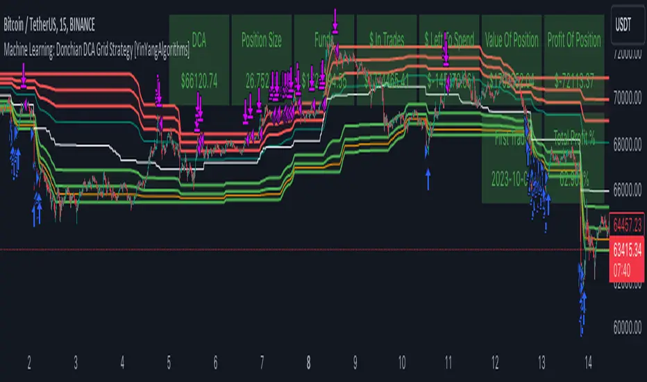
Machine Learning: Donchian DCA Grid Strategy [YinYangAlgorithms]This strategy uses a Machine Learning approach on the Donchian Channels with a DCA and Grid purchase/sell Strategy. Not only that, but it uses a custom Bollinger calculation to determine its Basis which is used as a mild sell location. This strategy is a pure DCA strategy in the sense that no shorts are used and theoretically it can be used in webhooks on most exchanges as it’s only using Spot Orders. The idea behind this strategy is we utilize both the Highest Highs and Lowest Lows within a Machine Learning standpoint to create Buy and Sell zones. We then fraction these zones off into pieces to create Grids. This allows us to ‘micro’ purchase as it enters these zones and likewise ‘micro’ sell as it goes up into the upper (sell) zones.
You have the option to set how many grids are used, by default we use 100 with max 1000. These grids can be ‘stacked’ together if a single bar is to go through multiple at the same time. For instance, if a bar goes through 30 grids in one bar, it will have a buy/sell power of 30x. Stacking Grid Buy and (sometimes) Sells is a very crucial part of this strategy that allows it to purchase multitudes during crashes and capitalize on sales during massive pumps.
With the grids, you’ll notice there is a middle line within the upper and lower part that makes the grid. As a Purchase Type within our Settings this is identified as ‘Middle of Zone Purchase Amount In USDT’. The middle of the grid may act as the strongest grid location (aside from maybe the bottom). Therefore there is a specific purchase amount for this Grid location.
This DCA Strategy also features two other purchase methods. Most importantly is its ‘Purchase More’ type. Essentially it will attempt to purchase when the Highest High or Lowest Low moves outside of the Outer band. For instance, the Lowest Low becomes Lower or the Higher High becomes Higher. When this happens may be a good time to buy as it is featuring a new High or Low over an extended period.
The last but not least Purchase type within this Strategy is what we call a ‘Strong Buy’. The reason for this is its verified by the following:
The outer bounds have been pushed (what causes a ‘Purchase More’)
The Price has crossed over the EMA 21
It has been verified through MACD, RSI or MACD Historical (Delta) using Regular and Hidden Divergence (Note, only 1 of these verifications is required and it can be any).
By default we don’t have Purchase Amount for ‘Strong Buy’ set, but that doesn’t mean it can’t be viable, it simply means we have only seen a few pairs where it actually proved more profitable allocating money there rather than just increasing the purchase amount for ‘Purchase More’ or ‘Grids’.
Now that you understand where we BUY, we should discuss when we SELL.
This Strategy features 3 crucial sell locations, and we will discuss each individually as they are very important.
1. ‘Sell Some At’: Here there are 4 different options, by default its set to ‘Both’ but you can change it around if you want. Your options are:
‘Both’ - You will sell some at both locations. The amount sold is the % used at ‘Sell Some %’.
‘Basis Line’ - You will sell some when the price crosses over the Basis Line. The amount sold is the % used at ‘Sell Some %’.
‘Percent’ - You will sell some when the Close is >= X% between the Lower Inner and Upper Inner Zone.
‘None’ - This simply means don’t ever Sell Some.
2. Sell Grids. Sell Grids are exactly like purchase grids and feature the same amount of grids. You also have the ability to ‘Stack Grid Sells’, which basically means if a bar moves multiple grids, it will stack the amount % wise you will sell, rather than just selling the default amount. Sell Grids use a DCA logic but for selling, which we deem may help adjust risk/reward ratio for selling, especially if there is slow but consistent bullish movement. It causes these grids to constantly push up and therefore when the close is greater than them, accrue more profit.
3. Take Profit. Take profit occurs when the close first goes above the Take Profit location (Teal Line) and then Closes below it. When Take Profit occurs, ALL POSITIONS WILL BE SOLD. What may happen is the price enters the Sell Grid, doesn’t go all the way to the top ‘Exiting it’ and then crashes back down and closes below the Take Profit. Take Profit is a strong location which generally represents a strong profit location, and that a strong momentum has changed which may cause the price to revert back to the buy grid zone.
Keep in mind, if you have (by default) ‘Only Sell If Profit’ toggled, all sell locations will only create sell orders when it is profitable to do so. Just cause it may be a good time to sell, doesn’t mean based on your DCA it is. In our opinion, only selling when it is profitable to do so is a key part of the DCA purchase strategy.
You likewise have the ability to ‘Only Buy If Lower than DCA’, which is likewise by default. These two help keep the Yin and Yang by balancing each other out where you’re only purchasing and selling when it makes logical sense too, even if that involves ignoring a signal and waiting for a better opportunity.
Tutorial:
Like most of our Strategies, we try to capitalize on lower Time Frames, generally the 15 minutes so we may find optimal entry and exit locations while still maintaining a strong correlation to trend patterns.
First off, let’s discuss examples of how this Strategy works prior to applying Machine Learning (enabled by default).
In this example above we have disabled the showing of ‘Potential Buy and Sell Signals’ so as to declutter the example. In here you can see where actual trades had gone through for both buying and selling and get an idea of how the strategy works. We also have disabled Machine Learning for this example so you can see the hard lines created by the Donchian Channel. You can also see how the Basis line ‘white line’ may act as a good location to ‘Sell Some’ and that it moves quite irregularly compared to the Donchian Channel. This is due to the fact that it is based on two custom Bollinger Bands to create the basis line.
Here we zoomed out even further and moved back a bit to where there were dense clusters of buy and sell orders. Sometimes when the price is rather volatile you’ll see it ‘Ping Pong’ back and forth between the buy and sell zones quite quickly. This may be very good for your trades and profit as a whole, especially if ‘Only Buy If Lower Than DCA’ and ‘Only Sell If Profit’ are both enabled; as these toggles will ensure you are:
Always lowering your Average when buying
Always making profit when selling
By default 8% commission is added to the Strategy as well, to simulate the cost effects of if these trades were taking place on an actual exchange.
In this example we also turned on the visuals for our ‘Purchase More’ (orange line) and ‘Take Profit’ (teal line) locations. These are crucial locations. The Purchase More makes purchases when the bottom of the grid has been moved (may dictate strong price movement has occurred and may be potential for correction). Our Take Profit may help secure profit when a momentum change is happening and all of the Sell Grids weren’t able to be used.
In the example above we’ve enabled Buy and Sell Signals so that you can see where the Take Profit and Purchase More signals have occurred. The white circle demonstrates that not all of the Position Size was sold within the Sell Grids, and therefore it was ALL CLOSED when the price closed below the Take Profit Line (Teal).
Then, when the bottom of the Donchian Channel was pushed further down due to the close (within the yellow circle), a Purchase More Signal was triggered.
When the close keeps pushing the bottom of the Buy Grid lower, it can cause multiple Purchase More Signals to occur. This is normal and also a crucial part of this strategy to help lower your DCA. Please note, the Purchase More won’t trigger a Buy if the Close is greater than the DCA and you have ‘Only Purchase If Lower Than DCA’ activated.
By turning on Machine Learning (default settings) the Buy and Sell Grid Zones are smoothed out more. It may cause it to look quite a bit different. Machine Learning although it looks much worse, may help increase the profit this Strategy can produce. Previous results DO NOT mean future results, but in this example, prior to turning on Machine Learning it had produced 37% Profit in ~5 months and with Machine Learning activated it is now up to 57% Profit in ~5 months.
Machine Learning causes the Strategy to focus less on Grids and more on Purchase More when it comes to getting its entries. However, if you likewise attempt to focus on Purchase More within non Machine Learning, the locations are different and therefore the results may not be as profitable.
PLEASE NOTE:
By default this strategy uses 1,000,000 as its initial capital. The amount it purchases in its Settings is relevant to this Initial capital. Considering this is a DCA Strategy, we only want to ‘Micro’ Buy and ‘Micro’ Sell whenever conditions are met.
Therefore, if you increase the Initial Capital, you’ll likewise want to increase the Purchase Amounts within the Settings and Vice Versa. For instance, if you wish to set the Initial Capital to 10,000, you should likewise can the amounts in the Settings to 1% of what they are to account for this.
We may change the Purchase Amounts to be based on %’s in a later update if it is requested.
We will conclude this Tutorial here, hopefully you can see how a DCA Grid Purchase Model applied to Machine Learning Donchian Channels may be useful for making strategic purchases in low and high zones.
Settings:
Display Data:
Show Potential Buy Locations: These locations are where 'Potentially' orders can be placed. Placement of orders is dependant on if you have 'Only Buy If Lower Than DCA' toggled and the Price is lower than DCA. It also is effected by if you actually have any money left to purchase with; you can't buy if you have no money left!
Show Potential Sell Locations: These locations are where 'Potentially' orders will be sold. If 'Only Sell If Profit' is toggled, the sell will only happen if you'll make profit from it!
Show Grid Locations: Displaying won't affect your trades but it can be useful to see where trades will be placed, as well as which have gone through and which are left to be purchased. Max 100 Grids, but visuals will only be shown if its 20 or less.
Purchase Settings:
Only Buy if its lower than DCA: Generally speaking, we want to lower our Average, and therefore it makes sense to only buy when the close is lower than our current DCA and a Purchase Condition is met.
Compound Purchases: Compounding Purchases means reinvesting profit back into your trades right away. It drastically increases profits, but it also increases risk too. It will adjust your Purchase Amounts for the Purchase Type you have set at the same % rate of strategy initial_capital to the amounts you have set.
Adjust Purchase Amount Ratio to Maintain Risk level: By adjusting purchase levels we generally help maintain a safe risk level. Basically we generally want to reserve X amount of % for each purchase type being used and relocate money when there is too much in one type. This helps balance out purchase amounts and ensure the types selected have a correct ratio to ensure they can place the right amount of orders.
Stack Grid Buys: Stacking Buy Grids is when the Close crosses multiple Buy Grids within the same bar. Should we still only purchase the value of 1 Buy Grid OR stack the grid buys based on how many buy grids it went through.
Purchase Type: Where do you want to make Purchases? We recommend lowering your risk by combining All purchase types, but you may also customize your trading strategy however you wish.
Strong Buy Purchase Amount In USDT: How much do you want to purchase when the 'Strong Buy' signal appears? This signal only occurs after it has at least entered the Buy Zone and there have been other verifications saying it's now a good time to buy. Our Strong Buy Signal is a very strong indicator that a large price movement towards the Sell Zone will likely occur. It almost always results in it leaving the Buy Zone and usually will go to at least the White Basis line where you can 'Sell Some'.
Buy More Purchase Amount In USDT: How much should you purchase when the 'Purchase More' signal appears? This 'Purchase More' signal occurs when the lowest level of the Buy Zone moves lower. This is a great time to buy as you're buying the dip and generally there is a correction that will allow you to 'Sell Some' for some profit.
Amount of Grid Buy and Sells: How many Grid Purchases do you want to make? We recommend having it at the max of 10, as it will essentially get you a better Average Purchase Price, but you may adjust it to whatever you wish. This amount also only matters if your Purchase Type above incorporates Grid Purchases. Max 100 Grids, but visuals will only be shown if it's 20 or less.
Each Grid Purchase Amount In USDT: How much should you purchase after closing under a grid location? Keep in mind, if you have 10 grids and it goes through each, it will be this amount * 10. Grid purchasing is a great way to get a good entry, lower risk and also lower your average.
Middle Of Zone Purchase Amount In USDT: The Middle Of Zone is the strongest grid location within the Buy Zone. This is why we have a unique Purchase Amount for this Grid specifically. Please note you need to have 'Middle of Zone is a Grid' enabled for this Purchase Amount to be used.
Sell:
Only Sell if its Profit: There is a chance that during a dump, all your grid buys when through, and a few Purchase More Signals have appeared. You likely got a good entry. A Strong Buy may also appear before it starts to pump to the Sell Zone. The issue that may occur is your Average Purchase Price is greater than the 'Sell Some' price and/or the Grids in the Sell Zone and/or the Strong Sell Signal. When this happens, you can either take a loss and sell it, or you can hold on to it and wait for more purchase signals to therefore lower your average more so you can take profit at the next sell location. Please backtest this yourself within our YinYang Purchase Strategy on the pair and timeframe you are wanting to trade on. Please also note, that previous results will not always reflect future results. Please assess the risk yourself. Don't trade what you can't afford to lose. Sometimes it is better to strategically take a loss and continue on making profit than to stay in a bad trade for a long period of time.
Stack Grid Sells: Stacking Sell Grids is when the Close crosses multiple Sell Grids within the same bar. Should we still only sell the value of 1 Sell Grid OR stack the grid sells based on how many sell grids it went through.
Stop Loss Type: This is when the Close has pushed the Bottom of the Buy Grid More. Do we Stop Loss or Purchase More?? By default we recommend you stay true to the DCA part of this strategy by Purchasing More, but this is up to you.
Sell Some At: Where if selected should we 'Sell Some', this may be an important way to sell a little bit at a good time before the price may correct. Also, we don't want to sell too much incase it doesn't correct though, so its a 'Sell Some' location. Basis Line refers to our Moving Basis Line created from 2 Bollinger Bands and Percent refers to a Percent difference between the Lower Inner and Upper Inner bands.
Sell Some At Percent Amount: This refers to how much % between the Lower Inner and Upper Inner bands we should well at if we chose to 'Sell Some'.
Sell Some Min %: This refers to the Minimum amount between the Lower Inner band and Close that qualifies a 'Sell Some'. This acts as a failsafe so we don't 'Sell Some' for too little.
Sell % At Strong Sell Signal: How much do we sell at the 'Strong Sell' Signal? It may act as a strong location to sell, but likewise Grid Sells could be better.
Grid and Donchian Settings:
Donchian Channel Length: How far back are we looking back to determine our Donchian Channel.
Extra Outer Buy Width %: How much extra should we push the Outer Buy (Low) Width by?
Extra Inner Buy Width %: How much extra should we push the Inner Buy (Low) Width by?
Extra Inner Sell Width %: How much extra should we push the Inner Sell (High) Width by?
Extra Outer Sell Width %: How much extra should we push the Outer Sell (High) Width by?
Machine Learning:
Rationalized Source Type: Donchians usually use High/Low. What Source is our Rationalized Source using?
Machine Learning Type: Are we using a Simple ML Average, KNN Mean Average, KNN Exponential Average or None?
Machine Learning Length: How far back is our Machine Learning going to keep data for.
k-Nearest Neighbour (KNN) Length: How many k-Nearest Neighbours will we account for?
Fast ML Data Length: What is our Fast ML Length?? This is used with our Slow Length to create our KNN Distance.
Slow ML Data Length: What is our Slow ML Length?? This is used with our Fast Length to create our KNN Distance.
If you have any questions, comments, ideas or concerns please don't hesitate to contact us.
HAPPY TRADING!