Buscar en scripts para "200亿美元是多少人民币"
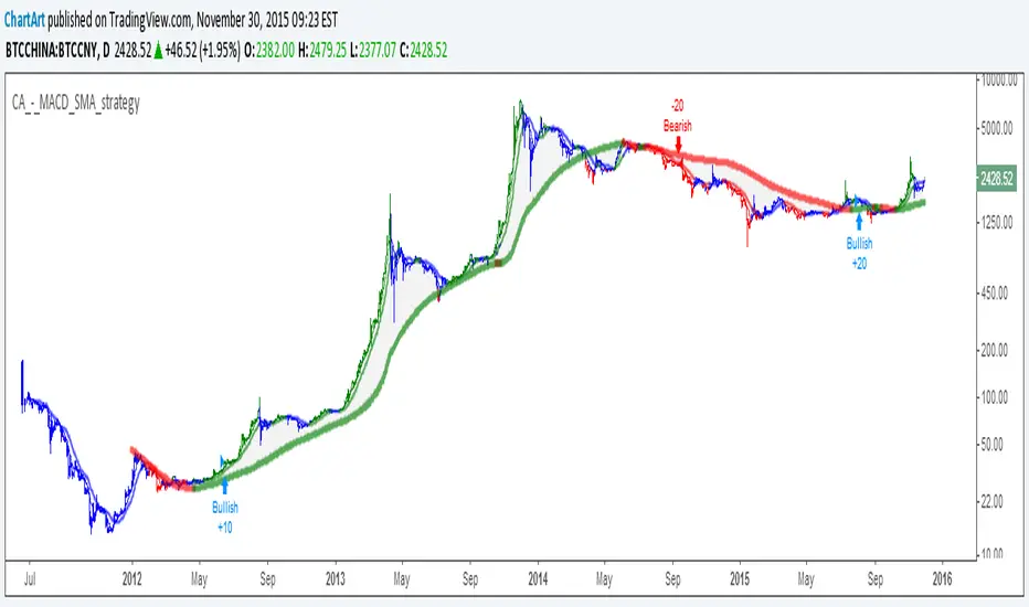
MACD + SMA 200 Strategy (by ChartArt)Here is a combination of the classic MACD (moving average convergence divergence indicator) with the classic slow moving average SMA with period 200 together as a strategy.
This strategy goes long if the MACD histogram and the MACD momentum are both above zero and the fast MACD moving average is above the slow MACD moving average. As additional long filter the recent price has to be above the SMA 200. If the inverse logic is true, the strategy goes short. For the worst case there is a max intraday equity loss of 50% filter.
Save another $999 bucks with my free strategy.
This strategy works in the backtest on the daily chart of Bitcoin, as well as on the S&P 500 and the Dow Jones Industrial Average daily charts. Current performance as of November 30, 2015 on the SPX500 CFD daily is percent profitable: 68% since the year 1970 with a profit factor of 6.4. Current performance as of November 30, 2015 on the DOWI index daily is percent profitable: 51% since the year 1915 with a profit factor of 10.8.
All trading involves high risk; past performance is not necessarily indicative of future results. Hypothetical or simulated performance results have certain inherent limitations. Unlike an actual performance record, simulated results do not represent actual trading. Also, since the trades have not actually been executed, the results may have under- or over-compensated for the impact, if any, of certain market factors, such as lack of liquidity. Simulated trading programs in general are also subject to the fact that they are designed with the benefit of hindsight. No representation is being made that any account will or is likely to achieve profits or losses similar to those shown.

LONG TERM INVESTMENT TECHNICAL STRATEGY SCRIPT200 - WEEKLY MOVING AVERAGE
GREEN LINE IS 200 WEEKS MOVING AVERAGE OF CLOSE
BLUE LINE IS 200 WEEKS MOVING AVERAGE OF LOW MULTIPLIED BY 0.90
RED LINE IS 100 WEEKS MOVING AVERAGE OF CLOSE
CONDITION: GREEN LINE SHOULD BE ABOVE RED LINE AND PRICE SHOULD BE ABOVE GREEN LINE
BUY ONCE THE PRICE IS ABOVE GREEN LINE AND FULFILLS THE CONDITION.
TARGET 1 FOR TIME FRAME 1 YEAR= 2 X GREEN LINE VALUE WHEN PRICE CROSSED IT
TARGET 2 FOR TIME FRAME 3 YEARS= 3 X GREEN LINE VALUE WHEN PRICE CROSSED IT
TARGET 3 FOR TIME FRAME 5 YEARS= 5 X GREEN LINE VALUE WHEN PRICE CROSSED IT
TARGET 4 FOR TIME FRAME 10 YEARS= 10 X GREEN LINE VALUE WHEN PRICE CROSSED IT
STOP LOSS IS TRAILING TO BLUE LINE

200 SMA with EMA Ribbon (Custom Colors)Simple Moving Average with the longer- time based line analyzing both shorter and longer trends

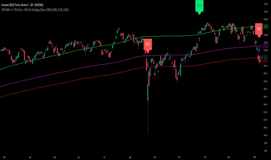
200 SMA (5%/-3% Buffer) for SPY & QQQ In my testing TQQQ is an absolute monster of an ETF that performs extremely well even from a buy and hold standpoint over long periods of time, its largest drawback is the massive drawdown exposure that it faces which can be easily sidestepped with this strategy.
This strategy is meant to basically abuse TQQQ's insane outperformance while augmenting the typical 200SMA strategy in a way that uses all of its strengths while avoiding getting whipsawed in sideways markets.
The strategy BUYS when price crosses 5% over the 200SMA and then SELLS when price drops 3% below the 200SMA. Between trades I'll be parking my entire account in SGOV.
So maximizing profit while minimizing risk.
You use the strategy based off of QQQ and then make the trades on TQQQ when it tells you to BUY/SELL.
Here are some reasons why I will be using this strategy:
Simple emotionless BUY and SELL signals where I don't care who the president is, what is happening in the world, who is bombing who, who the leadership team is, no attachment to individual companies and diversified across the NASDAQ.
~85% win percentage and when it does lose the loses are nothing compared to the wins and after a loss you're basically set up for a massive win in the next trade.
Max drawdown of around 53% when using TQQQ
You benefit massively when the market is doing well and when there is a recession you basically sit in SGOV for a year and then are set up for a monster recovery with a clear easy BUY signal. So as long as you're patient you win regardless of what happens.
The trades are often very long term resulting in you taking advantage of Long Term Capital Gains tax advantage which could mean saving up to 15-20% in taxes.
With only a few trades you can spend time doing other stuff and don't have to track or pay attention to anything that is happening.
Simple, easy, and massively profitable.
200 Week Moving Average HeatmapСolors part of the SMA depending on the change in % (delta %) to the previous value. From blue(none to low increase) through green(moderate increase) to red(high increase).

200/150
This a variation to my 120/60 Trend Model for the daily chart on Bitcoin, which has quite reliably been determining the over all trend as well as low risk entries within a longer term trend. It's a combination of 150 & 220 SMA, used on the 1D chart. Once price closes below both SMAs trend is an early bearish signal, while the SMAs flipping to red is later but more reliable bearish signal. For bullish trend it is the same thing just the opposite. Once the "cloud" switches red trend is bearish while once it switches green it's bullish.
Bitcoin tends to get rejected by the cloud during bullish and bearish trends. Once Bitcoin pushes through the cloud the trend will typically reverse.
Bitcoin trading within or close to the cloud is generally a good long or short entries, depending on the color of the cloud (red: short & green: long).

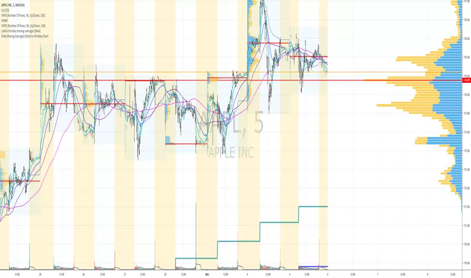
Daily Moving Averages (EMAs + SMAs) to Intraday Chart200 SMA, 100 SMA, 50 EMA, and 20 EMA daily averages to intraday chart
Roshan Dash Ultimate Trading DashboardHas the key moving averages sma (10,20,50,200) in daily and above timeframe. And for lower timeframe it has ema (10,20,50,200) and vwap. Displays key information like marketcap, sector, lod%, atr, atr% and distance of atr from 50sma . All things which help determine whether or not to take trade.

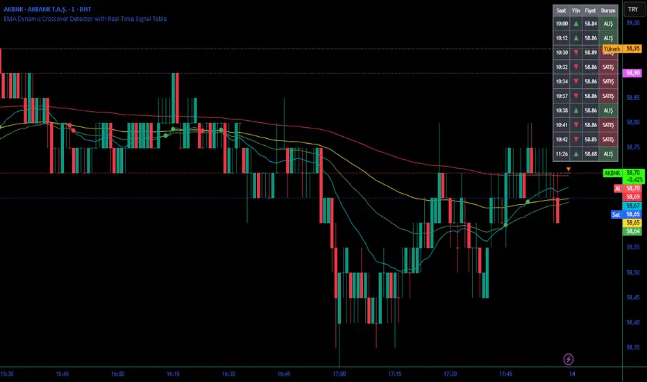
EMA Dynamic Crossover Detector with Real-Time Signal TableDescriptionWhat This Indicator Does:This indicator monitors all possible crossovers between four key exponential moving averages (20, 50, 100, and 200 periods) and displays them both visually on the chart and in an organized data table. Unlike standard EMA indicators that only plot the lines, this tool actively detects every crossover event, marks the exact crossover point with a circle, records the precise price level, and maintains a running log of all crossovers during the trading session. It's designed for traders who want comprehensive EMA crossover analysis without manually watching multiple moving average pairs.Key Features:
Four Essential EMAs: Plots 20, 50, 100, and 200-period exponential moving averages with color-coded thin lines for clean chart presentation
Complete Crossover Detection: Monitors all 6 possible EMA pair combinations (20×50, 20×100, 20×200, 50×100, 50×200, 100×200) in both directions
Precise Price Marking: Places colored circles at the exact average price where crossovers occur (not just at candle close)
Real-Time Signal Table: Displays up to 10 most recent crossovers with timestamp, direction, exact price, and signal type
Session Filtering: Only records crossovers during active trading hours (10:00-18:00 Istanbul time) to avoid noise from low-liquidity periods
Automatic Daily Reset: Clears the signal table at the start of each new trading day for fresh analysis
Built-In Alerts: Two alert conditions (bullish and bearish crossovers) that can be configured to send notifications
How It Works:The indicator calculates four exponential moving averages using the standard EMA formula, then continuously monitors for crossover events using Pine Script's ta.crossover() and ta.crossunder() functions:Bullish Crossovers (Green ▲):
When a faster EMA crosses above a slower EMA, indicating potential upward momentum:
20 crosses above 50, 100, or 200
50 crosses above 100 or 200
100 crosses above 200 (Golden Cross when it's the 50×200)
Bearish Crossovers (Red ▼):
When a faster EMA crosses below a slower EMA, indicating potential downward momentum:
20 crosses below 50, 100, or 200
50 crosses below 100 or 200
100 crosses below 200 (Death Cross when it's the 50×200)
Price Calculation:
Instead of marking crossovers at the candle's close price (which might not be where the actual cross occurred), the indicator calculates the average price between the two crossing EMAs, providing a more accurate representation of the crossover point.Signal Table Structure:The table in the top-right corner displays four columns:
Saat (Time): Exact time of crossover in HH:MM format
Yön (Direction): Arrow indicator (▲ green for bullish, ▼ red for bearish)
Fiyat (Price): Calculated average price at the crossover point
Durum (Status): Signal classification ("ALIŞ" for buy signals, "SATIŞ" for sell signals) with color-coded background
The table shows up to 10 most recent crossovers, automatically updating as new signals appear. If no crossovers have occurred during the session within the time filter, it displays "Henüz kesişim yok" (No crossovers yet).EMA Color Coding:
EMA 20 (Aqua/Turquoise): Fastest-reacting, most sensitive to recent price changes
EMA 50 (Green): Short-term trend indicator
EMA 100 (Yellow): Medium-term trend indicator
EMA 200 (Red): Long-term trend baseline, key support/resistance level
How to Use:For Day Traders:
Monitor 20×50 crossovers for quick entry/exit signals within the day
Use the time filter (10:00-18:00) to focus on high-volume trading hours
Check the signal table throughout the session to track momentum shifts
Look for confirmation: if 20 crosses above 50 and price is above EMA 200, bullish bias is stronger
For Swing Traders:
Focus on 50×200 crossovers (Golden Cross/Death Cross) for major trend changes
Use higher timeframes (4H, Daily) for more reliable signals
Wait for price to close above/below the crossover point before entering
Combine with support/resistance levels for better entry timing
For Position Traders:
Monitor 100×200 crossovers on daily/weekly charts for long-term trend changes
Use as confirmation of major market shifts
Don't react to every crossover—wait for sustained movement after the cross
Consider multiple timeframe analysis (if crossovers align on weekly and daily, signal is stronger)
Understanding EMA Hierarchies:The indicator becomes most powerful when you understand EMA relationships:Bullish Hierarchy (Strongest to Weakest):
All EMAs ascending (20 > 50 > 100 > 200): Strong uptrend
20 crosses above 50 while both are above 200: Pullback ending in uptrend
50 crosses above 200 while 20/50 below: Early trend reversal signal
Bearish Hierarchy (Strongest to Weakest):
All EMAs descending (20 < 50 < 100 < 200): Strong downtrend
20 crosses below 50 while both are below 200: Rally ending in downtrend
50 crosses below 200 while 20/50 above: Early trend reversal signal
Trading Strategy Examples:Pullback Entry Strategy:
Identify major trend using EMA 200 (price above = uptrend, below = downtrend)
Wait for pullback (20 crosses below 50 in uptrend, or above 50 in downtrend)
Enter when 20 re-crosses 50 in the trend direction
Place stop below/above the recent swing point
Exit when 20 crosses 50 against the trend again
Golden Cross/Death Cross Strategy:
Wait for 50×200 crossover (appears in the signal table)
Verify: Check if crossover occurs with increasing volume
Entry: Enter in the direction of the cross after a pullback
Stop: Place stop below/above the 200 EMA
Target: Swing high/low or when opposite crossover occurs
Multi-Crossover Confirmation:
Watch for multiple crossovers in the same direction within a short period
Example: 20×50 crossover followed by 20×100 = strengthening momentum
Enter after the second confirmation crossover
More crossovers = stronger signal but also means you're entering later
Time Filter Benefits:The 10:00-18:00 Istanbul time filter prevents recording crossovers during:
Pre-market volatility and gaps
Low-volume overnight sessions (for 24-hour markets)
After-hours erratic movements
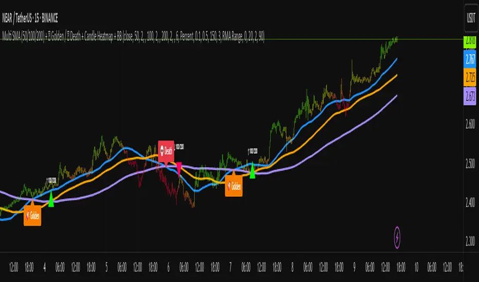
Multi SMA + Golden/Death + Heatmap + BB**Multi SMA (50/100/200) + Golden/Death + Candle Heatmap + BB**
A practical trend toolkit that blends classic 50/100/200 SMAs with clear crossover labels, special 🚀 Golden / 💀 Death Cross markers, and a readable candle heatmap based on a dynamic regression midline and volatility bands. Optional Bollinger Bands are included for context.
* See trend direction at a glance with SMAs.
* Get minimal, de-cluttered labels on important crosses (50↔100, 50↔200, 100↔200).
* Highlight big regime shifts with special Golden/Death tags.
* Read momentum and volatility with the candle heatmap.
* Add Bollinger Bands if you want classic mean-reversion context.
Designed to be lightweight, non-repainting on confirmed bars, and flexible across timeframes.
# What This Indicator Does (plain English)
* **Tracks trend** using **SMA 50/100/200** and lets you optionally compute each SMA on a higher or different timeframe (HTF-safe, no lookahead).
* **Prints labels** when SMAs cross each other (up or down). You can force signals only after bar close to avoid repaint.
* **Marks Golden/Death Crosses** (50 over/under 200) with special labels so major regime changes stand out.
* **Colors candles** with a **heatmap** built from a regression midline and volatility bands—greenish above, reddish below, with a smooth gradient.
* **Optionally shows Bollinger Bands** (basis SMA + stdev bands) and fills the area between them.
* **Includes alert conditions** for Golden and Death Cross so you can automate notifications.
---
# Settings — Simple Explanations
## Source
* **Source**: Price source used to calculate SMAs and Bollinger basis. Default: `close`.
## SMA 50
* **Show 50**: Turn the SMA(50) line on/off.
* **Length 50**: How many bars to average. Lower = faster but noisier.
* **Color 50** / **Width 50**: Visual style.
* **Timeframe 50**: Optional alternate timeframe for SMA(50). Leave empty to use the chart timeframe.
## SMA 100
* **Show 100**: Turn the SMA(100) line on/off.
* **Length 100**: Bars used for the mid-term trend.
* **Color 100** / **Width 100**: Visual style.
* **Timeframe 100**: Optional alternate timeframe for SMA(100).
## SMA 200
* **Show 200**: Turn the SMA(200) line on/off.
* **Length 200**: Bars used for the long-term trend.
* **Color 200** / **Width 200**: Visual style.
* **Timeframe 200**: Optional alternate timeframe for SMA(200).
## Signals (crossover labels)
* **Show crossover signals**: Prints triangle labels on SMA crosses (50↔100, 50↔200, 100↔200).
* **Wait for bar close (confirmed)**: If ON, signals only appear after the candle closes (reduces repaint).
* **Min bars between same-pair signals**: Minimum spacing to avoid duplicate labels from the same SMA pair too often.
* **Trend filter (buy: 50>100>200, sell: 50<100<200)**: Only show bullish labels when SMAs are stacked bullish (50 above 100 above 200), and only show bearish labels when stacked bearish.
### Label Offset
* **Offset mode**: Choose how to push labels away from price:
* **Percent**: Offset is a % of price.
* **ATR x**: Offset is ATR(14) × multiplier.
* **Percent of price (%)**: Used when mode = Percent.
* **ATR multiplier (for ‘ATR x’)**: Used when mode = ATR x.
### Label Colors
* **Bull color** / **Bear color**: Background of triangle labels.
* **Bull label text color** / **Bear label text color**: Text color inside the triangles.
## Golden / Death Cross
* **Show 🚀 Golden Cross (50↑200)**: Show a special “Golden” label when SMA50 crosses above SMA200.
* **Golden label color** / **Golden text color**: Styling for Golden label.
* **Show 💀 Death Cross (50↓200)**: Show a special “Death” label when SMA50 crosses below SMA200.
* **Death label color** / **Death text color**: Styling for Death label.
## Candle Heatmap
* **Enable heatmap candle colors**: Turns the heatmap on/off.
* **Length**: Lookback for the regression midline and volatility measure.
* **Deviation Multiplier**: Band width around the midline (bigger = wider).
* **Volatility basis**:
* **RMA Range** (smoothed high-low range)
* **Stdev** (standard deviation of close)
* **Upper/Middle/Lower color**: Gradient colors for the heatmap.
* **Heatmap transparency (0..100)**: 0 = solid, 100 = invisible.
* **Force override base candles**: Repaint base candles so heatmap stays visible even if your chart has custom coloring.
## Bollinger Bands (optional)
* **Show Bollinger Bands**: Toggle the overlay on/off.
* **Length**: Basis SMA length.
* **StdDev Multiplier**: Distance of bands from the basis in standard deviations.
* **Basis color** / **Band color**: Line colors for basis and bands.
* **Bands fill transparency**: Opacity of the fill between upper/lower bands.
---
# Features & How It Works
## 1) HTF-Safe SMAs
Each SMA can be calculated on the chart timeframe or a higher/different timeframe you choose. The script pulls HTF values **without lookahead** (non-repainting on confirmed bars).
## 2) Crossover Labels (Three Pairs)
* **50↔100**, **50↔200**, **100↔200**:
* **Triangle Up** label when the first SMA crosses **above** the second.
* **Triangle Down** label when it crosses **below**.
* Optional **Trend Filter** ensures only signals aligned with the overall stack (50>100>200 for bullish, 50<100<200 for bearish).
* **Debounce** spacing avoids repeated labels for the same pair too close together.
## 3) Golden / Death Cross Highlights
* **🚀 Golden Cross**: SMA50 crosses **above** SMA200 (often a longer-term bullish regime shift).
* **💀 Death Cross**: SMA50 crosses **below** SMA200 (often a longer-term bearish regime shift).
* Separate styling so they stand out from regular cross labels.
## 4) Candle Heatmap
* Builds a **regression midline** with **volatility bands**; colors candles by their position inside that channel.
* Smooth gradient: lower side → reddish, mid → yellowish, upper side → greenish.
* Helps you see momentum and “where price sits” relative to a dynamic channel.
## 5) Bollinger Bands (Optional)
* Classic **basis SMA** ± **StdDev** bands.
* Light visual context for mean-reversion and volatility expansion.
## 6) Alerts
* **Golden Cross**: `🚀 GOLDEN CROSS: SMA 50 crossed ABOVE SMA 200`
* **Death Cross**: `💀 DEATH CROSS: SMA 50 crossed BELOW SMA 200`
Add these to your alerts to get notified automatically.
---
# Tips & Notes
* For fewer false positives, keep **“Wait for bar close”** ON, especially on lower timeframes.
* Use the **Trend Filter** to align signals with the broader stack and cut noise.
* For HTF context, set **Timeframe 50/100/200** to higher frames (e.g., H1/H4/D) while you trade on a lower frame.
* Heatmap “Length” and “Deviation Multiplier” control smoothness and channel width—tune for your asset’s volatility.
Support and resistance levels (Day, Week, Month) + EMAs + SMAs(ENG): This Pine 5 script provides various tools for configuring and displaying different support and resistance levels, as well as moving averages (EMA and SMA) on charts. Using these tools is an essential strategy for determining entry and exit points in trades.
Support and Resistance Levels
Daily, weekly, and monthly support and resistance levels play a key role in analyzing price movements:
Daily levels: Represent prices where a cryptocurrency has tended to bounce within the current trading day.
Weekly levels: Reflect strong prices that hold throughout the week.
Monthly levels: Indicate the most significant levels that can influence price movement over the month.
When trading cryptocurrencies, traders use these levels to make decisions about entering or exiting positions. For example, if a cryptocurrency approaches a weekly resistance level and fails to break through it, this may signal a sell opportunity. If the price reaches a daily support level and starts to bounce up, it may indicate a potential long position.
Market context and trading volumes are also important when analyzing support and resistance levels. High volume near a level can confirm its significance and the likelihood of subsequent price movement. Traders often combine analysis across different time frames to get a more complete picture and improve the accuracy of their trading decisions.
Moving Averages
Moving averages (EMA and SMA) are another important tool in the technical analysis of cryptocurrencies:
EMA (Exponential Moving Average): Gives more weight to recent prices, allowing it to respond more quickly to price changes.
SMA (Simple Moving Average): Equally considers all prices over a given period.
Key types of moving averages used by traders:
EMA 50 and 200: Often used to identify trends. The crossing of the 50-day EMA with the 200-day EMA is called a "golden cross" (buy signal) or a "death cross" (sell signal).
SMA 50, 100, 150, and 200: These periods are often used to determine long-term trends and support/resistance levels. Similar to the EMA, the crossings of these averages can signal potential trend changes.
Settings Groups:
EMA Golden Cross & Death Cross: A setting to display the "golden cross" and "death cross" for the EMA.
EMA 50 & 200: A setting to display the 50-day and 200-day EMA.
Support and Resistance Levels: Includes settings for daily, weekly, and monthly levels.
SMA 50, 100, 150, 200: A setting to display the 50, 100, 150, and 200-day SMA.
SMA Golden Cross & Death Cross: A setting to display the "golden cross" and "death cross" for the SMA.
Components:
Enable/disable the display of support and resistance levels.
Show level labels.
Parameters for adjusting offset, display of EMA and SMA, and their time intervals.
Parameters for configuring EMA and SMA Golden Cross & Death Cross.
EMA Parameters:
Enable/disable the display of 50 and 200-day EMA.
Color and style settings for EMA.
Options to use bar gaps and the "LookAhead" function.
SMA Parameters:
Enable/disable the display of 50, 100, 150, and 200-day SMA.
Color and style settings for SMA.
Options to use bar gaps and the "LookAhead" function.
Effective use of support and resistance levels, as well as moving averages, requires an understanding of technical analysis, discipline, and the ability to adapt the strategy according to changing market conditions.
(RUS) Данный Pine 5 скрипт предоставляет разнообразные инструменты для настройки и отображения различных уровней поддержки и сопротивления, а также скользящих средних (EMA и SMA) на графиках. Использование этих инструментов является важной стратегией для определения точек входа и выхода из сделок.
Уровни поддержки и сопротивления
Дневные, недельные и месячные уровни поддержки и сопротивления играют ключевую роль в анализе движения цен:
Дневные уровни: Представляют собой цены, на которых криптовалюта имела тенденцию отскакивать в течение текущего торгового дня.
Недельные уровни: Отражают сильные цены, которые сохраняются в течение недели.
Месячные уровни: Указывают на наиболее значимые уровни, которые могут влиять на движение цены в течение месяца.
При торговле криптовалютами трейдеры используют эти уровни для принятия решений о входе в позицию или закрытии сделки. Например, если криптовалюта приближается к недельному уровню сопротивления и не удается его преодолеть, это может стать сигналом для продажи. Если цена достигает дневного уровня поддержки и начинает отскакивать вверх, это может указывать на возможность открытия длинной позиции.
Контекст рынка и объемы торговли также важны при анализе уровней поддержки и сопротивления. Высокий объем при приближении к уровню может подтвердить его значимость и вероятность последующего движения цены. Трейдеры часто комбинируют анализ различных временных рамок для получения более полной картины и улучшения точности своих торговых решений.
Скользящие средние
Скользящие средние (EMA и SMA) являются еще одним важным инструментом в техническом анализе криптовалют:
EMA (Exponential Moving Average): Экспоненциальная скользящая средняя, которая придает большее значение последним ценам. Это позволяет более быстро реагировать на изменения в ценах.
SMA (Simple Moving Average): Простая скользящая средняя, которая равномерно учитывает все цены в заданном периоде.
Основные виды скользящих средних, которые используются трейдерами:
EMA 50 и 200: Часто используются для выявления трендов. Пересечение 50-дневной EMA с 200-дневной EMA называется "золотым крестом" (сигнал на покупку) или "крестом смерти" (сигнал на продажу).
SMA 50, 100, 150 и 200: Эти периоды часто используются для определения долгосрочных трендов и уровней поддержки/сопротивления. Аналогично EMA, пересечения этих средних могут сигнализировать о возможных изменениях тренда.
Группы настроек:
EMA Golden Cross & Death Cross: Настройка для отображения "золотого креста" и "креста смерти" для EMA.
EMA 50 & 200: Настройка для отображения 50-дневной и 200-дневной EMA.
Уровни поддержки и сопротивления: Включает настройки для дневных, недельных и месячных уровней.
SMA 50, 100, 150, 200: Настройка для отображения 50, 100, 150 и 200-дневных SMA.
SMA Golden Cross & Death Cross: Настройка для отображения "золотого креста" и "креста смерти" для SMA.
Компоненты:
Включение/отключение отображения уровней поддержки и сопротивления.
Показ ярлыков уровней.
Параметры для настройки смещения, отображения EMA и SMA, а также их временных интервалов.
Параметры для настройки EMA и SMA Golden Cross & Death Cross.
Параметры EMA:
Включение/отключение отображения 50 и 200-дневных EMA.
Настройки цвета и стиля для EMA.
Опции для использования разрыва баров и функции "LookAhead".
Параметры SMA:
Включение/отключение отображения 50, 100, 150 и 200-дневных SMA.
Настройки цвета и стиля для SMA.
Опции для использования разрыва баров и функции "LookAhead".
Эффективное использование уровней поддержки и сопротивления, а также скользящих средних, требует понимания технического анализа, дисциплины и умения адаптировать стратегию в зависимости от изменяющихся условий рынка.

QTrade Golden, Bronze & Death, Bubonic Cross AlertsThis indicator highlights key EMA regime shifts with simple, color-coded triangles:
- Golden / Death Cross — 50 EMA crossing above/below the 200 EMA.
- Bronze / Bubonic Cross — 50 EMA crossing above/below the 100 EMA.
- Early-Warning Proxy — tiny triangles for the 4 EMA vs. 200 EMA (4↑200 and 4↓200). These often fire before the 50/100 and 50/200 crosses.
No text clutter on the chart—just triangles. Colors: gold (50↑200), red (50↓200), darker-yellow bronze (50↑100), burgundy (50↓100), turquoise (4↑200), purple (4↓200).
What it tells you (in order of warning → confirmation)
- First warning: 4 EMA crosses the 200 EMA (proxy for price shifting around the 200 line).
- Second warning: 50 EMA crosses the 100 EMA (Bronze/Bubonic).
- Confirmation: 50 EMA crosses the 200 EMA (Golden/Death).
Alerts included
- Golden Cross (50↑200) and Death Cross (50↓200)
- Bronze Cross (50↑100) and Bubonic Cross (50↓100)
- 4 EMA vs. 200 EMA crosses (up & down) — early-warning proxy
- Price–100 EMA events (touch/cross, if enabled in settings)

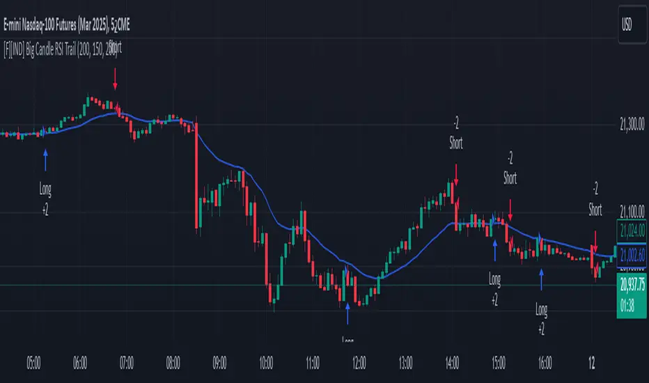
Big Candle Identifier with RSI Divergence and Advanced Stops1. Strategy Objective
The main goal of this strategy is to:
Identify significant price momentum (big candles).
Enter trades at opportune moments based on market signals (candlestick patterns and RSI divergence).
Limit initial risk through a fixed stop loss.
Maximize profits by using a trailing stop that activates only after the trade moves a specified distance in the profitable direction.
2. Components of the Strategy
A. Big Candle Identification
The strategy identifies big candles as indicators of strong momentum.
A big candle is defined as:
The body (absolute difference between close and open) of the current candle (body0) is larger than the bodies of the last five candles.
The candle is:
Bullish Big Candle: If close > open.
Bearish Big Candle: If open > close.
Purpose: Big candles signal potential continuation or reversal of trends, serving as the primary entry trigger.
B. RSI Divergence
Relative Strength Index (RSI): A momentum oscillator used to detect overbought/oversold conditions and divergence.
Fast RSI: A 5-period RSI, which is more sensitive to short-term price movements.
Slow RSI: A 14-period RSI, which smoothens fluctuations over a longer timeframe.
Divergence: The difference between the fast and slow RSIs.
Positive divergence (divergence > 0): Bullish momentum.
Negative divergence (divergence < 0): Bearish momentum.
Visualization: The divergence is plotted on the chart, helping traders confirm momentum shifts.
C. Stop Loss
Initial Stop Loss:
When entering a trade, an immediate stop loss of 200 points is applied.
This stop loss ensures the maximum risk is capped at a predefined level.
Implementation:
Long Trades: Stop loss is set below the entry price at low - 200 points.
Short Trades: Stop loss is set above the entry price at high + 200 points.
Purpose:
Prevents significant losses if the price moves against the trade immediately after entry.
D. Trailing Stop
The trailing stop is a dynamic risk management tool that adjusts with price movements to lock in profits. Here’s how it works:
Activation Condition:
The trailing stop only starts trailing when the trade moves 200 ticks (profit) in the right direction:
Long Position: close - entry_price >= 200 ticks.
Short Position: entry_price - close >= 200 ticks.
Trailing Logic:
Once activated, the trailing stop:
For Long Positions: Trails behind the price by 150 ticks (trail_stop = close - 150 ticks).
For Short Positions: Trails above the price by 150 ticks (trail_stop = close + 150 ticks).
Exit Condition:
The trade exits automatically if the price touches the trailing stop level.
Purpose:
Ensures profits are locked in as the trade progresses while still allowing room for price fluctuations.
E. Trade Entry Logic
Long Entry:
Triggered when a bullish big candle is identified.
Stop loss is set at low - 200 points.
Short Entry:
Triggered when a bearish big candle is identified.
Stop loss is set at high + 200 points.
F. Trade Exit Logic
Trailing Stop: Automatically exits the trade if the price touches the trailing stop level.
Fixed Stop Loss: Exits the trade if the price hits the predefined stop loss level.
G. 21 EMA
The strategy includes a 21-period Exponential Moving Average (EMA), which acts as a trend filter.
EMA helps visualize the overall market direction:
Price above EMA: Indicates an uptrend.
Price below EMA: Indicates a downtrend.
H. Visualization
Big Candle Identification:
The open and close prices of big candles are plotted for easy reference.
Trailing Stop:
Plotted on the chart to visualize its progression during the trade.
Green Line: Indicates the trailing stop for long positions.
Red Line: Indicates the trailing stop for short positions.
RSI Divergence:
Positive divergence is shown in green.
Negative divergence is shown in red.
3. Key Parameters
trail_start_ticks: The number of ticks required before the trailing stop activates (default: 200 ticks).
trail_distance_ticks: The distance between the trailing stop and price once the trailing stop starts (default: 150 ticks).
initial_stop_loss_points: The fixed stop loss in points applied at entry (default: 200 points).
tick_size: Automatically calculates the minimum tick size for the trading instrument.
4. Workflow of the Strategy
Step 1: Entry Signal
The strategy identifies a big candle (bullish or bearish).
If conditions are met, a trade is entered with a fixed stop loss.
Step 2: Initial Risk Management
The trade starts with an initial stop loss of 200 points.
Step 3: Trailing Stop Activation
If the trade moves 200 ticks in the profitable direction:
The trailing stop is activated and follows the price at a distance of 150 ticks.
Step 4: Exit the Trade
The trade is exited if:
The price hits the trailing stop.
The price hits the initial stop loss.
5. Advantages of the Strategy
Risk Management:
The fixed stop loss ensures that losses are capped.
The trailing stop locks in profits after the trade becomes profitable.
Momentum-Based Entries:
The strategy uses big candles as entry triggers, which often indicate strong price momentum.
Divergence Confirmation:
RSI divergence helps validate momentum and avoid false signals.
Dynamic Profit Protection:
The trailing stop adjusts dynamically, allowing the trade to capture larger moves while protecting gains.
6. Ideal Market Conditions
This strategy performs best in:
Trending Markets:
Big candles and momentum signals are more effective in capturing directional moves.
High Volatility:
Larger price swings improve the probability of reaching the trailing stop activation level (200 ticks).
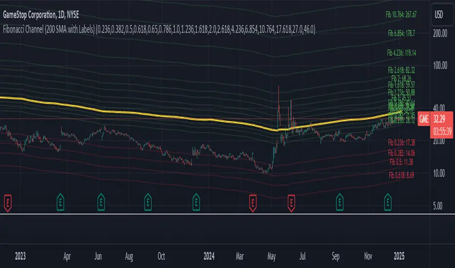
Fibonacci Channel Standard Deviation levels based off 200MAThis script dynamically combines Fibonacci levels with the 200-period simple moving average (SMA), offering a powerful tool for identifying high-probability support and resistance zones. By adjusting to the changing 200 SMA, the script remains relevant across different market phases.
Key Features:
Dynamic Fibonacci Levels:
The script automatically calculates Fibonacci retracements and extensions relative to the 200 SMA.
These levels adapt to market trends, offering more relevant zones compared to static Fibonacci tools.
Support and Resistance Zones:
In uptrends, price often respects retracement levels above the 200 SMA (e.g., 38.2%, 50%, 61.8%).
In downtrends, price may interact with retracements and extensions below the 200 SMA (e.g., 23.6%, 1.618).
Customizable Confluence Zones:
Key levels such as the golden pocket (61.8%–65%) are highlighted as high-probability zones for reversals or continuations.
Extensions (e.g., 1.618) can serve as profit targets or bearish continuation points.
Practical Applications:
Identifying Reversal Zones:
Look for confluence between Fibonacci levels and the 200 SMA to identify potential reversal points.
Example: A pullback to the 61.8%–65% golden pocket near the 200 SMA often signals a bullish reversal.
Trend Confirmation:
In uptrends, price respecting Fibonacci retracements above the 200 SMA (e.g., 38.2%, 50%) confirms strength.
Use Fibonacci extensions (e.g., 1.618) as profit targets during strong trends.
Dynamic Risk Management:
Place stop-losses just below key Fibonacci retracement levels near the 200 SMA to minimize risk.
Bearish Scenarios:
Below the 200 SMA, Fibonacci retracements and extensions act as resistance levels and bearish targets.
How to Use:
Volume Confirmation: Watch for volume spikes near Fibonacci levels to confirm support or resistance.
Price Action: Combine with candlestick patterns (e.g., engulfing candles, pin bars) for precise entries.
Trend Indicators: Use in conjunction with shorter moving averages or RSI to confirm market direction.
Example Setup:
Scenario: Price retraces to the 61.8% Fibonacci level while holding above the 200 SMA.
Confirmation: Volume spikes, and a bullish engulfing candle forms.
Action: Enter long with a stop-loss just below the 200 SMA and target extensions like 1.618.
Key Takeaways:
The 200 SMA serves as a reliable long-term trend anchor.
Fibonacci retracements and extensions provide dynamic zones for trade entries, exits, and risk management.
Combining this tool with volume, price action, or other indicators enhances its effectiveness.
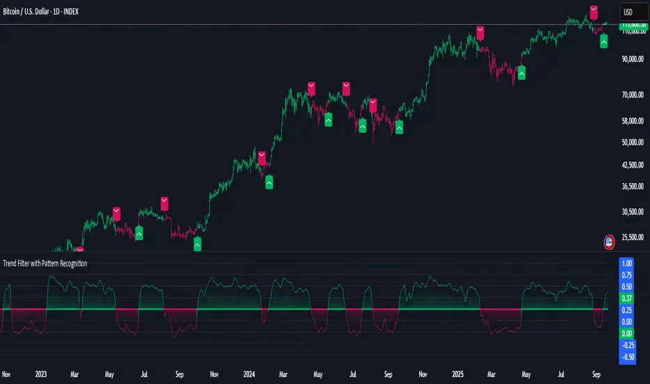
Wavelet-Trend ML Integration [Alpha Extract]Alpha-Extract Volatility Quality Indicator
The Alpha-Extract Volatility Quality (AVQ) Indicator provides traders with deep insights into market volatility by measuring the directional strength of price movements. This sophisticated momentum-based tool helps identify overbought and oversold conditions, offering actionable buy and sell signals based on volatility trends and standard deviation bands.
🔶 CALCULATION
The indicator processes volatility quality data through a series of analytical steps:
Bar Range Calculation: Measures true range (TR) to capture price volatility.
Directional Weighting: Applies directional bias (positive for bullish candles, negative for bearish) to the true range.
VQI Computation: Uses an exponential moving average (EMA) of weighted volatility to derive the Volatility Quality Index (VQI).
Smoothing: Applies an additional EMA to smooth the VQI for clearer signals.
Normalization: Optionally normalizes VQI to a -100/+100 scale based on historical highs and lows.
Standard Deviation Bands: Calculates three upper and lower bands using standard deviation multipliers for volatility thresholds.
Signal Generation: Produces overbought/oversold signals when VQI reaches extreme levels (±200 in normalized mode).
Formula:
Bar Range = True Range (TR)
Weighted Volatility = Bar Range × (Close > Open ? 1 : Close < Open ? -1 : 0)
VQI Raw = EMA(Weighted Volatility, VQI Length)
VQI Smoothed = EMA(VQI Raw, Smoothing Length)
VQI Normalized = ((VQI Smoothed - Lowest VQI) / (Highest VQI - Lowest VQI) - 0.5) × 200
Upper Band N = VQI Smoothed + (StdDev(VQI Smoothed, VQI Length) × Multiplier N)
Lower Band N = VQI Smoothed - (StdDev(VQI Smoothed, VQI Length) × Multiplier N)
🔶 DETAILS
Visual Features:
VQI Plot: Displays VQI as a line or histogram (lime for positive, red for negative).
Standard Deviation Bands: Plots three upper and lower bands (teal for upper, grayscale for lower) to indicate volatility thresholds.
Reference Levels: Horizontal lines at 0 (neutral), +100, and -100 (in normalized mode) for context.
Zone Highlighting: Overbought (⋎ above bars) and oversold (⋏ below bars) signals for extreme VQI levels (±200 in normalized mode).
Candle Coloring: Optional candle overlay colored by VQI direction (lime for positive, red for negative).
Interpretation:
VQI ≥ 200 (Normalized): Overbought condition, strong sell signal.
VQI 100–200: High volatility, potential selling opportunity.
VQI 0–100: Neutral bullish momentum.
VQI 0 to -100: Neutral bearish momentum.
VQI -100 to -200: High volatility, strong bearish momentum.
VQI ≤ -200 (Normalized): Oversold condition, strong buy signal.
🔶 EXAMPLES
Overbought Signal Detection: When VQI exceeds 200 (normalized), the indicator flags potential market tops with a red ⋎ symbol.
Example: During strong uptrends, VQI reaching 200 has historically preceded corrections, allowing traders to secure profits.
Oversold Signal Detection: When VQI falls below -200 (normalized), a lime ⋏ symbol highlights potential buying opportunities.
Example: In bearish markets, VQI dropping below -200 has marked reversal points for profitable long entries.
Volatility Trend Tracking: The VQI plot and bands help traders visualize shifts in market momentum.
Example: A rising VQI crossing above zero with widening bands indicates strengthening bullish momentum, guiding traders to hold or enter long positions.
Dynamic Support/Resistance: Standard deviation bands act as dynamic volatility thresholds during price movements.
Example: Price reversals often occur near the third standard deviation bands, providing reliable entry/exit points during volatile periods.
🔶 SETTINGS
Customization Options:
VQI Length: Adjust the EMA period for VQI calculation (default: 14, range: 1–50).
Smoothing Length: Set the EMA period for smoothing (default: 5, range: 1–50).
Standard Deviation Multipliers: Customize multipliers for bands (defaults: 1.0, 2.0, 3.0).
Normalization: Toggle normalization to -100/+100 scale and adjust lookback period (default: 200, min: 50).
Display Style: Switch between line or histogram plot for VQI.
Candle Overlay: Enable/disable VQI-colored candles (lime for positive, red for negative).
The Alpha-Extract Volatility Quality Indicator empowers traders with a robust tool to navigate market volatility. By combining directional price range analysis with smoothed volatility metrics, it identifies overbought and oversold conditions, offering clear buy and sell signals. The customizable standard deviation bands and optional normalization provide precise context for market conditions, enabling traders to make informed decisions across various market cycles.
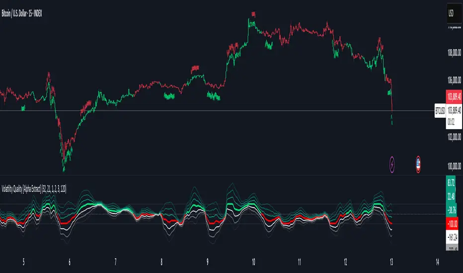
Volatility Quality [Alpha Extract]The Alpha-Extract Volatility Quality (AVQ) Indicator provides traders with deep insights into market volatility by measuring the directional strength of price movements. This sophisticated momentum-based tool helps identify overbought and oversold conditions, offering actionable buy and sell signals based on volatility trends and standard deviation bands.
🔶 CALCULATION
The indicator processes volatility quality data through a series of analytical steps:
Bar Range Calculation: Measures true range (TR) to capture price volatility.
Directional Weighting: Applies directional bias (positive for bullish candles, negative for bearish) to the true range.
VQI Computation: Uses an exponential moving average (EMA) of weighted volatility to derive the Volatility Quality Index (VQI).
vqiRaw = ta.ema(weightedVol, vqiLen)
Smoothing: Applies an additional EMA to smooth the VQI for clearer signals.
Normalization: Optionally normalizes VQI to a -100/+100 scale based on historical highs and lows.
Standard Deviation Bands: Calculates three upper and lower bands using standard deviation multipliers for volatility thresholds.
vqiStdev = ta.stdev(vqiSmoothed, vqiLen)
upperBand1 = vqiSmoothed + (vqiStdev * stdevMultiplier1)
upperBand2 = vqiSmoothed + (vqiStdev * stdevMultiplier2)
upperBand3 = vqiSmoothed + (vqiStdev * stdevMultiplier3)
lowerBand1 = vqiSmoothed - (vqiStdev * stdevMultiplier1)
lowerBand2 = vqiSmoothed - (vqiStdev * stdevMultiplier2)
lowerBand3 = vqiSmoothed - (vqiStdev * stdevMultiplier3)
Signal Generation: Produces overbought/oversold signals when VQI reaches extreme levels (±200 in normalized mode).
Formula:
Bar Range = True Range (TR)
Weighted Volatility = Bar Range × (Close > Open ? 1 : Close < Open ? -1 : 0)
VQI Raw = EMA(Weighted Volatility, VQI Length)
VQI Smoothed = EMA(VQI Raw, Smoothing Length)
VQI Normalized = ((VQI Smoothed - Lowest VQI) / (Highest VQI - Lowest VQI) - 0.5) × 200
Upper Band N = VQI Smoothed + (StdDev(VQI Smoothed, VQI Length) × Multiplier N)
Lower Band N = VQI Smoothed - (StdDev(VQI Smoothed, VQI Length) × Multiplier N)
🔶 DETAILS
Visual Features:
VQI Plot: Displays VQI as a line or histogram (lime for positive, red for negative).
Standard Deviation Bands: Plots three upper and lower bands (teal for upper, grayscale for lower) to indicate volatility thresholds.
Reference Levels: Horizontal lines at 0 (neutral), +100, and -100 (in normalized mode) for context.
Zone Highlighting: Overbought (⋎ above bars) and oversold (⋏ below bars) signals for extreme VQI levels (±200 in normalized mode).
Candle Coloring: Optional candle overlay colored by VQI direction (lime for positive, red for negative).
Interpretation:
VQI ≥ 200 (Normalized): Overbought condition, strong sell signal.
VQI 100–200: High volatility, potential selling opportunity.
VQI 0–100: Neutral bullish momentum.
VQI 0 to -100: Neutral bearish momentum.
VQI -100 to -200: High volatility, strong bearish momentum.
VQI ≤ -200 (Normalized): Oversold condition, strong buy signal.
🔶 EXAMPLES
Overbought Signal Detection: When VQI exceeds 200 (normalized), the indicator flags potential market tops with a red ⋎ symbol.
Example: During strong uptrends, VQI reaching 200 has historically preceded corrections, allowing traders to secure profits.
Oversold Signal Detection: When VQI falls below -200 (normalized), a lime ⋏ symbol highlights potential buying opportunities.
Example: In bearish markets, VQI dropping below -200 has marked reversal points for profitable long entries.
Volatility Trend Tracking: The VQI plot and bands help traders visualize shifts in market momentum.
Example: A rising VQI crossing above zero with widening bands indicates strengthening bullish momentum, guiding traders to hold or enter long positions.
Dynamic Support/Resistance: Standard deviation bands act as dynamic volatility thresholds during price movements.
Example: Price reversals often occur near the third standard deviation bands, providing reliable entry/exit points during volatile periods.
🔶 SETTINGS
Customization Options:
VQI Length: Adjust the EMA period for VQI calculation (default: 14, range: 1–50).
Smoothing Length: Set the EMA period for smoothing (default: 5, range: 1–50).
Standard Deviation Multipliers: Customize multipliers for bands (defaults: 1.0, 2.0, 3.0).
Normalization: Toggle normalization to -100/+100 scale and adjust lookback period (default: 200, min: 50).
Display Style: Switch between line or histogram plot for VQI.
Candle Overlay: Enable/disable VQI-colored candles (lime for positive, red for negative).
The Alpha-Extract Volatility Quality Indicator empowers traders with a robust tool to navigate market volatility. By combining directional price range analysis with smoothed volatility metrics, it identifies overbought and oversold conditions, offering clear buy and sell signals. The customizable standard deviation bands and optional normalization provide precise context for market conditions, enabling traders to make informed decisions across various market cycles.
Market Breadth Peaks & Troughs IndicatorIndicator Overview
Market Breadth (S5TH) visualizes extremes of market strength and weakness by overlaying -
a 200-period EMA (long-term trend)
a 5-period EMA (short-term trend, user-adjustable)
on the percentage of S&P 500 constituents trading above their 200-day SMA (INDEX:S5TH).
Peaks (▼) and troughs (▲) are detected with prominence filters so you can quickly spot overbought and oversold conditions.
⸻
1. Core Logic
Component Description
Breadth series INDEX:S5TH — % of S&P 500 stocks above their 200-SMA
Long EMA 200-EMA to capture the primary trend
Short EMA 5-EMA (default, editable) for short-term swings
Peak detection ta.pivothigh + prominence ⇒ major peaks marked with red ▼
Trough detection (200 EMA) ta.pivotlow + prominence + value < longTroughLvl ⇒ blue ▲
Trough detection (5 EMA) ta.pivotlow + prominence + value < shortTroughLvl ⇒ green ▲
Background shading Pink when 200 EMA slope is down and 5 EMA sits below 200 EMA
⸻
2. Adjustable Parameters (input())
Group Variable Default Purpose
Symbol breadthSym INDEX:S5TH Breadth index
Long EMA longLen 200 Period of long EMA
Short EMA shortLen 5 Period of short EMA
Pivot width (long) pivotLen 20 Bars left/right for 200-EMA peaks/troughs
Pivot width (short) pivotLenS 10 Bars for 5-EMA troughs
Prominence (long) promThresh 0.5 %-pt Depth filter for 200-EMA pivots
Prominence (short) promThreshS 3.0 %-pt Depth filter for 5-EMA pivots
Trough level (long) longTroughLvl 50 % Max value to accept a 200-EMA trough
Trough level (short) shortTroughLvl 30 % Max value to accept a 5-EMA trough
⸻
3. Signal Guide
Marker / Color Meaning Typical reading
Red ▼ Major breadth peak Overbought / possible top
Blue ▲ Deep 200-EMA trough End of mid-term correction
Green ▲ Shallow 5-EMA trough (early) Short-term rebound setup
Pink background Long-term down-trend and short-term weak Risk-off phase
⸻
4. Typical Use Cases
1. Counter-trend timing
• Fade greed: trim longs on red ▼
• Buy fear: scale in on green ▲; add on blue ▲
2. Trend filter
• Avoid new longs while the background is pink; wait for a trough & recovery.
3. Risk management
• Reduce exposure when peaks appear, reload partial size on confirmed troughs.
⸻
5. Notes & Tips
• INDEX:S5TH is sourced from TradingView and may be back-adjusted when index membership changes.
• Fine-tune pivotLen, promThresh, and level thresholds to match current volatility before relying on alerts or automated rules.
• Slope thresholds (±0.10 %-pt) that trigger background shading can also be customized for different market regimes.

Stochastic RSI Strategy with Inverted Trend LogicOverview:
The Stochastic RSI Strategy with Inverted Trend Logic is a custom-built Pine Script indicator that leverages the Stochastic RSI and a 200-period moving average to generate precise buy and sell signals. It is specifically designed for traders looking to capture opportunities during short-term market movements while factoring in broader trend conditions.
Key Components:
Stochastic RSI:
Stochastic RSI is a momentum indicator that applies stochastic calculations to the standard Relative Strength Index (RSI), rather than price data. This makes it particularly sensitive to market momentum changes, which is essential for timing entries and exits.
K Line and D Line: The indicator calculates and smooths both the K and D lines to capture momentum shifts more accurately.
200-Period Moving Average:
The 200-period Simple Moving Average (SMA) is used as a trend filter.
If the price is above the 200-period SMA, the trend is considered bullish.
If the price is below the 200-period SMA, the trend is considered bearish.
Inverted Trading Logic:
The trading logic is inverted from traditional strategies:
Long trades are executed only when the market is in a bearish trend (price below the 200-period moving average).
Short trades are executed only when the market is in a bullish trend (price above the 200-period moving average).
This inversion allows traders to take advantage of potential trend reversals by entering positions in the opposite direction of the prevailing trend.
Trading Rules:
Long Trade Conditions (Buy Signal):
The Stochastic RSI K line must be below 5 for 4 consecutive candles (oversold condition).
The price must be below the 200-period SMA (indicating a bearish trend).
Once these conditions are met, the indicator will generate a buy signal on the close of the 4th candle.
Exit Condition: The long position is exited when the Stochastic RSI K line crosses above 50 (neutral level).
Short Trade Conditions (Sell Signal):
The Stochastic RSI K line must be above 95 for 4 consecutive candles (overbought condition).
The price must be above the 200-period SMA (indicating a bullish trend).
Once these conditions are met, the indicator will generate a sell signal on the close of the 4th candle.
Exit Condition: The short position is exited when the Stochastic RSI K line crosses below 50.
Visual Signals on the Chart:
Buy Signal:
A green triangle below the bar is displayed on the chart when a buy condition is met, indicating a potential long trade opportunity.
The text "BUY" is displayed for further clarity.
Sell Signal:
A red triangle above the bar is displayed on the chart when a sell condition is met, indicating a potential short trade opportunity.
The text "SELL" is displayed for further clarity.
How to Use the Indicator:
Attach the Indicator: Apply the indicator to your desired chart (works on any time frame, but is optimized for short- to medium-term trading).
Monitor Signals: Watch for buy and sell signals on the chart:
Buy Signal: Enter long positions when a green triangle appears below the candle.
Sell Signal: Enter short positions when a red triangle appears above the candle.
Exit Positions: Exit long positions when the Stochastic RSI crosses above the 50 level, and exit short positions when the Stochastic RSI crosses below the 50 level.
Indicator Display:
Stochastic RSI: A visual representation of the Stochastic RSI (K and D lines) is plotted below the price chart, with overbought (100), midpoint (50), and oversold (0) levels clearly marked.
200-period SMA: The 200-period moving average is plotted on the price chart, giving a clear indication of the broader trend direction (orange line).
Key Benefits:
Reversal Opportunities: This strategy allows traders to capture reversal trades by using an inverted logic where longs are taken in bearish conditions and shorts are taken in bullish conditions. This can help capitalize on potential trend exhaustion and reversals.
Clear and Simple Rules: The use of Stochastic RSI and the 200-period moving average ensures the strategy remains simple yet effective, making it easy for traders to follow.
Visual Alerts: The indicator provides clear buy and sell signals, making it easy for traders to spot trading opportunities in real-time without needing to monitor multiple conditions manually.
Limitations and Considerations:
Trend Changes: Since the strategy is designed to work during trend reversals, it might not perform as well during strong, prolonged trends where price continues moving in one direction without significant pullbacks.
Time Frame Suitability: While the indicator works on any time frame, shorter time frames may result in more frequent signals and higher trade frequency, whereas higher time frames will provide fewer but potentially stronger signals.
Conclusion:
The Stochastic RSI Strategy with Inverted Trend Logic is a powerful tool for traders looking to capture market reversals by entering trades against the prevailing trend direction based on momentum exhaustion. Its simple and clear logic, combined with easy-to-understand visual signals, makes it a versatile indicator for both novice and experienced traders.

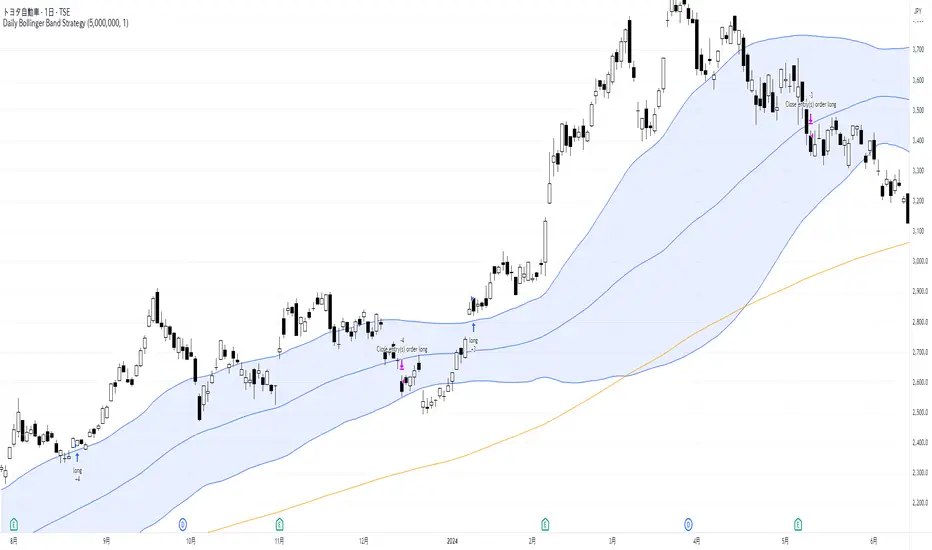
Daily Bollinger Band StrategyOverview of the Daily Bollinger Band Strategy
1. Strategy Overview and Features
This strategy is a tool for backtesting a trading method that uses Bollinger Bands. It is *not* a tool for automated trading.
1-1. Main Display Items
The main chart displays the Bollinger Bands and the 200-day moving average.
It also shows the entry and exit points along with the position size (in units of 100 shares).
1-2. Summary of Trading Rules
For long (buy) strategies, the trade enters when the price crosses above the +1σ line of the Bollinger Bands, aiming to ride an upward trend. The position is exited when the price crosses below the middle band.
For short (sell) strategies, the trade enters when the price crosses below the -1σ line of the Bollinger Bands, aiming to ride a downward trend. The position is exited when the price crosses above the middle band.
1-3. Strategic Enhancements
The strategy uses the slope of the 200-day moving average to determine the trend direction and enter trades accordingly. This improves the win rate and payoff ratio.
Additionally, to reduce the probability of ruin, the risk per trade is limited to 1.0% of capital, and position sizing is adjusted using ATR (a volatility indicator).
2. Trading Rules
2-1. Chart Type
Only daily charts are used.
2-2. Indicators Used
(1) Bollinger Bands** (used for entry and exit signals)
- Period: Fixed at 80 days
- Upper and lower bands: Fixed at ±1σ
(2) Moving Average** (used to determine trend direction)
- Period: Fixed at 200 days
- Trend direction is judged based on whether the difference from the previous day is positive (upward) or negative (downward)
2-3. Buy Rules
Setup:
- Price crosses above the +1σ line from below
- Both the middle band and 200-day moving average are upward sloping
Entry:
- Buy at the next day’s market open using a market order
Exit:
- If the price crosses below the middle band, sell at the next day’s open using a market order
2-4. Sell Rules
Setup:
- Price crosses below the -1σ line from above
- Both the middle band and 200-day moving average are downward sloping
Entry:
- Sell at the next day’s market open using a market order
Exit:
- If the price crosses above the middle band, buy back at the next day’s open using a market order
2-5. Risk Management Rules
- Risk per trade: 1.0% of total capital (acceptable loss = capital × 1.0%)
- Position size: Acceptable loss ÷ 2ATR (rounded down to the nearest unit of 100 shares)
2-6. Other Notes
- No brokerage fees
- No pyramiding
- No partial exits
- No reverse positions (no “stop-and-reverse” trades)
3. Strategy Parameters
The following settings can be specified:
3-1. Period Settings
- Start date: Set the start date for the backtest period
- Stop date: Set the end date for the backtest period
3-2. Display of Trend and Signals
- Show trend: When checked, the background color of the bars is light red for an uptrend and light blue for a downtrend
- Show signal: When checked, entry and exit signals are displayed (note: signals are executed at the next day’s open, so there is a one-day lag in the display)
3-3. Capital Management Settings
- Funds: Capital available for trading (in JPY)
- Risk rate: Specify what percentage of the capital to risk per trade
Settings in the “Properties” tab are not used in this strategy.
4. Backtest Results (Example)
Here are the backtest results conducted by the author:
- Target Stocks: All components of the Nikkei 225
- Test Period: January 4, 2000 – December 30, 2024
- Data Points: 12,886
- Win Rate: 33.45%
- Net Profit: ¥82,132,380
- Payoff Ratio: 2.450
- Expected Value: ¥6,373.8
- Risk Rate: 1.0%
- Probability of Ruin: 0.00%
---
デイリー・ボリンジャーバンド・ストラテジーの概要
1. ストラテジーの概要と特徴
このストラテジーは、ボリンジャーバンドを使ったトレード手法のバックテストを行うツールです。自動売買を行うツールではありません。
1-1. 主な表示項目
メインチャートにボリンジャーバンドと 200日移動平均線を表示します。
また、エントリーと手仕舞いのタイミングと数量(100株単位)も表示されます。
1-2. トレードルールの概要
買い戦略の場合、ボリンジャーバンドの +1σ 超えでエントリーして上昇トレンドに乗り、ミドルバンドを割ったら決済します。
売り戦略の場合、ボリンジャーバンドの -1σ 割りでエントリーして下降トレンドに乗り、ミドルバンドを上抜けたら決済します。
1-3. ストラテジーの工夫点
200日移動平均線の傾きを見てトレンド方向にエントリーをしています。こうして勝率とペイオフレシオの成績を向上しています。
また、破産確率を抑えるために、リスク資金比率を 1.0% にして、ATR(ボラティリティ指標) を使って注文数を調整しています。
2. 売買ルール
2-1. 使用するチャート
日足チャートに限定します
2-2. 使用する指標
(1) ボリンジャーバンド(仕掛けと手仕舞いのシグナルに使用)
期間は80日に固定
上下バンドは ±1σ に固定
(2) 移動平均線(トレンドの方向を見るために使用)
期間は200日に固定
移動平均の値の前日との差がプラスのとき上向き、マイナスのとき下向きと判断
2-3. 買いのルール
セットアップ:ボリンジャーバンドの +1σ を価格が下から上に交差 かつ ミドルバンドと 200日移動平均線が上向き
仕掛け:翌日の寄り付きに成行で買う
手仕舞い:ボリンジャーバンドのミドルバンドを価格が上から下に交差したら、翌日の寄り付きに成行で売る
2-4. 売りのルール
セットアップ:ボリンジャーバンドの -1σ を価格が上から下に交差 かつ ミドルバンドと 200日移動平均線が下向き
仕掛け:翌日の寄り付きに成行で売る
手仕舞い:ボリンジャーバンドのミドルバンドを価格が下から上に交差したら、翌日の寄り付きに成行で買い戻す
2-5. 資金管理のルール
リスク資金比率:資産の 1.0%(許容損失 = 資産 × 1.0%)
注文数:許容損失 ÷ 2ATR(単元株数未満は切り捨て)
2-6. その他
仲介手数料:なし
ピラミッディング:なし
分割決済:なし
ドテン:しない
3. ストラテジーのパラメーター
次の項目が指定できます。
3-1. 期間の設定
Staer date : バックテストの検証期間の開始日を指定します
Stop date : バックテストの検証期間の終了日を指定します
3-2. トレンドとシグナルの表示
Show trend : チェックを入れると、バーの背景色が、トレンドが上昇のときは薄い赤で、下落のときは薄い青で表示されます
Show signal : チェックを入れると、エントリーと手仕舞いのシグナルを表示します(シグナルの出た翌日の寄り付きに売買をするので表示に1日のずれがあります)
3-3. 資金管理用の設定
Funds : トレード用の資金(円)
Risk rate : 許容損失を資金の何%にするかで指定します
「プロパティタブ」で設定する値は、このストラテジーでは有効ではありません。
4. バックテストの結果(例)
作者がバックテストを実施した結果をお知らせします。
対象銘柄:日経225構成銘柄すべて
対象期間:2000年1月4日~2024年12月30日
データ件数:12,886
勝率:33.45%
純利益:82,132,380
ペイオフレシオ:2.450
期待値:6,373.8
リスク資金比率:1.0%
破産確率:0.00%
Pre-London High-Low Breakout IndicatorOverview
The Pre-London High-Low Breakout Indicator helps traders identify breakout opportunities at the London session open. It marks the high and low one hour before London opens (5 PM - 6 PM AEST) and incorporates a 200 SMA filter to confirm trade direction. The indicator also provides real-time breakout markers for precise entries.
How the Indicator Works
1. Pre-London High & Low Identification (5 PM - 6 PM AEST)
The indicator tracks the highest and lowest price levels within this period.
These levels act as key breakout zones once London opens.
The high and low remain visible until 12 AM AEST for reference.
2. 200 SMA as a Trend Filter
A 200 SMA (yellow, thick line) is plotted to filter breakout trades.
Only long (buy) trades are valid if price is above the 200 SMA.
Only short (sell) trades are valid if price is below the 200 SMA.
3. Real-Time Breakout Confirmation
Buy Signal (Green Diamond):
Price breaks above the pre-London high.
Price is above the 200 SMA.
Sell Signal (Red Diamond):
Price breaks below the pre-London low.
Price is below the 200 SMA.
No signal appears if the breakout is against the SMA trend, reducing false trades.
How to Use the Indicator Properly
Step 1: Identify the Pre-London Range (5 PM - 6 PM AEST)
Observe price movements and note the session high & low.
Do not take trades within this period—wait for a clear breakout.
Step 2: Wait for a Breakout After 6 PM AEST
A breakout must occur beyond the session high or low.
The breakout should be clear and decisive, not hovering around the range.
Step 3: Confirm with the 200 SMA
If price is above the 200 SMA, only buy signals are valid.
If price is below the 200 SMA, only sell signals are valid.
If a breakout occurs against the SMA, ignore it.
Step 4: Enter the Trade and Manage Risk
Enter the trade after the breakout candle closes.
Set stop-loss just inside the pre-London range to minimize risk.
Take profit using a 1:2 or 1:3 risk-reward ratio, or trail the stop.
Why This Strategy Works
Pre-London Liquidity Grab: Institutional traders set positions before the London open, making this range significant.
Trend Confirmation with SMA: Reduces false breakouts by filtering trades in the direction of the trend.
Real-Time Breakout Detection: Green and red diamond markers highlight valid breakouts that meet all conditions.
Final Notes
If price breaks out but quickly reverses, it may be a false breakout—avoid impulsive trades.
The indicator works best when combined with other confluences such as volume analysis or key support/resistance levels.
Alerts can be added to notify traders when a valid breakout occurs.
This setup is ideal for traders looking for a structured, rule-based approach to trading London session breakouts with a strong trend confirmation mechanism.
