VS Score [SpiritualHealer117]An experimental indicator that uses historical prices and readings of technical indicators to give the probability that stock and crypto prices will be in a certain range on the next close. This indicator may be helpful for options traders or for traders who want to see the probability of a move.
It classifies returns into five categories:
Extreme Rise - Over 2 standard deviations above normal returns
Rise - Between 0.5 standard deviations and 2 standard deviations above normal returns
Flat - Falling in the range of +/- 0.5 standard deviations of normal returns
Fall - Between 0.5 standard deviations and 2 standard deviations below normal returns
Extreme Fall - Over 2 standard deviations below normal returns
It is an adaptive probability model, which trains on the previous 1000 data points, and is calculated by creating probability vectors for the current reading of the PPO, MA, volume histogram, and previous return, and combining them into one probability vector.
Buscar en scripts para "通达信+选股公式+换手率+0.5+源码"

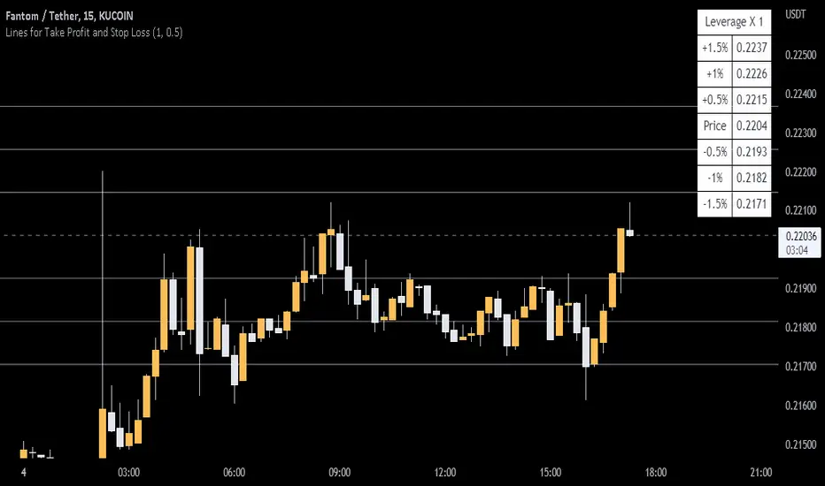
Lines and Table for risk managementABOUT THIS INDICATOR
This is a simple indicator that can help you manage the risk when you are trading, and especially if you are leverage trading. The indicator can also be used to help visualize and to find trades within a suitable or predefined trading range.
This script calculates and draws six “profit and risk lines” (levels) that show the change in percentage from the current price. The values are also shown in a table, to help you get a quick overview of risk before you trade.
ABOUT THE LINES/VALUES
This indicator draws seven percentage-lines, where the dotted line in the middle represents the current price. The other three lines on top of and below the middle line shows the different levels of change in percentage from current price (dotted line). The values are also shown in a table.
DEFAULT VALUES AND SETTINGS
By default the indicator draw lines 0.5%, 1.0%, and 1.5% from current price (step size = 0.5).
The default setting for leverage in this indicator = 1 (i.e. no leverage).
The line closest to dotted line (current price) is calculated by step size (%) * leverage (x) = % from price.
Pay attention to the %-values in the table, they represent the distance from the current price (dotted line) to where the lines are drawn.
* Be aware! If you change the leverage, the distance from the closest lines to the dotted line showing the current price increase.
SETTINGS
1. Leverage: set the leverage for what you are planning to trade on (1 = no leverage, 2 = 2 x leverage, 5 = 5 x leverage...).
2. Stepsize is used to set the distance between the lines and price.
EXAMPLES WITH DIFFERENT SETTINGS
1) Leverage = 1 (no leverage, default setting) and step size 0.5 (%). Lines plotted at (0.5%, 1%, 1.5%, and –0.5%, –1%, –1,5%) from the current price.
2) Leverage = 3 and stepsize 0.5(%). Lines plotted at (1.5%, 3.0%, 4.5%, and –1.5%, –3.0%, –4.5%) from the current price.
3) Leverage = 3 and stepsize 1(%). Lines plotted at (3%, 6%, 9%, and –3%, –6%, –9%) from the current price.
The distance to the nearest line from the current price is always calculated by the formula: Leverage * step size (%) = % to the nearest line from the current price.
Quantitative Backtesting Panel + ROI Table - ShortsThis script is an aggregate of a backtesting panel with quantitative metrics, ROI table and open ROI reader. It also contains a mechanism for having a fixed percentage stop loss, similar to native TV backtester. For shorts only.
Backtesting Panel:
- Certain metrics are color coded, with green being good performance, orange being neutral, red being undesirable.
• ROI : return with the system, in %
• ROI(COMP=1): return if money is compounded at a rate of 100%
• Hit rate: accuracy of the system, as a %
• Profit factor: gross profit/gross loss
• Maximum drawdown: the maximum value from a peak to a successive trough of the system's equity curve
• MAE: Maximum Adverse Excursion. The biggest loss of a trade suffered while the position is still open
• Total trades: total number of closed trades
• Max gain/max loss: shows the biggest win over the biggest loss suffered
• Sharpe ratio: measures the performance of the system with adjusted risk (no comparison to risk-free asset)
• CAGR: Compound Annual Growth Rate. The mean annual rate of growth of the system of n years (provided n>1)
• Kurtosis: measures how heavily the tails of the distribution differ from that of a normal distribution (symmetric on both sides of mean where mean=0, standard deviation=1). A normal distribution has a kurtosis of 3, and skewness of 0. The kurtosis indicates whether or not the tails of the returns contain extreme values
• Skewness: measures the symmetry of the distribution of returns
- Leptokurtic: K > 0. Having more kurtosis than a normal distribution. It's stretched up and to the side too (2nd pic down). High kurtosis (leptokurtic) is bad as the wider tails (called heavy tails) suggest there is relatively high probability of extreme events
- Mesokurtic: K =0. Having the same kurtosis as a normal distribution
- Platykurtic: K < 0. Having less kurtosis than a normal distribution. This suggests there are light tails and fewer extreme events in the distribution
- Skewness is good: +/- 0.5 (fairly symmetrical)
- Skewness is average: -1 to -0.5 or 0.5 to 1 (moderately skewed)
- Skewness is bad: > +/- 1 (highly skewed)
Evolving ROI table:
- The table of ROI values evolve with the year and month. The sum of each year is given. Please avoid using it on non-cryptocurrencies or any market whose trading session is not 24/7
Open ROI reader:
- At the top center is the open ROI of a trade

Quantitative Backtesting Panel + ROI Table - LongsThis script is an aggregate of a backtesting panel with quantitative metrics, ROI table and open ROI reader. It also contains a mechanism for having a fixed percentage stop loss, similar to native TV backtester. For longs only.
Backtesting Panel:
- Certain metrics are color coded, with green being good performance, orange being neutral, red being undesirable.
• ROI : return with the system, in %
• ROI(COMP=1): return if money is compounded at a rate of 100%
• Hit rate: accuracy of the system, as a %
• Profit factor: gross profit/gross loss
• Maximum drawdown: the maximum value from a peak to a successive trough of the system's equity curve
• MAE: Maximum Adverse Excursion. The biggest loss of a trade suffered while the position is still open
• Total trades: total number of closed trades
• Max gain/max loss: shows the biggest win over the biggest loss suffered
• Sharpe ratio: measures the performance of the system with adjusted risk (no comparison to risk-free asset)
• CAGR: Compound Annual Growth Rate. The mean annual rate of growth of the system of n years (provided n>1)
• Kurtosis: measures how heavily the tails of the distribution differ from that of a normal distribution (symmetric on both sides of mean where mean=0, standard deviation=1). A normal distribution has a kurtosis of 3, and skewness of 0. The kurtosis indicates whether or not the tails of the returns contain extreme values
• Skewness: measures the symmetry of the distribution of returns
- Leptokurtic: K > 0. Having more kurtosis than a normal distribution. It's stretched up and to the side too (2nd pic down). High kurtosis (leptokurtic) is bad as the wider tails (called heavy tails) suggest there is relatively high probability of extreme events
- Mesokurtic: K =0. Having the same kurtosis as a normal distribution
- Platykurtic: K < 0. Having less kurtosis than a normal distribution. This suggests there are light tails and fewer extreme events in the distribution
- Skewness is good: +/- 0.5 (fairly symmetrical)
- Skewness is average: -1 to -0.5 or 0.5 to 1 (moderately skewed)
- Skewness is bad: > +/- 1 (highly skewed)
Evolving ROI table:
- The table of ROI values evolve with the year and month. The sum of each year is given. Please avoid using it on non-cryptocurrencies or any market whose trading session is not 24/7
Open ROI reader:
- At the top center is the open ROI of a trade

American Approximation: Barone-Adesi and Whaley [Loxx]American Approximation: Barone-Adesi and Whaley is an American Options pricing model. This indicator also includes numerical greeks. You can compare the output of the American Approximation to the Black-Scholes-Merton value on the output of the options panel.
An American option can be exercised at any time up to its expiration date. This added freedom complicates the valuation of American options relative to their European counterparts. With a few exceptions, it is not possible to find an exact formula for the value of American options. Several researchers have, however, come up with excellent closed-form approximations. These approximations have become especially popular because they execute quickly on computers compared to numerical techniques. At the end of the chapter, we look at closed-form solutions for perpetual American options.
The Barone-Adesi and Whaley Approximation
The quadratic approximation method by Barone-Adesi and Whaley (1987) can be used to price American call and put options on an underlying asset with cost-of-carry rate b. When b > r, the American call value is equal to the European call value and can then be found by using the generalized Black-Scholes-Merton (BSM) formula. The model is fast and accurate for most practical input values.
American Call
C(S, C, T) = Cbsm(S, X, T) + A2 / (S/S*)^q2 ... when S < S*
C(S, C, T) = S - X ... when S >= S*
where Cbsm(S, X, T) is the general Black-Scholes-Merton call formula, and
A2 = S* / q2 * (1 - e^((b - r) * T)) * N(d1(S*)))
d1(S) = (log(S/X) + (b + v^2/2) * T) / (v * T^0.5)
q2 = (-(N-1) + ((N-1)^2 + 4M/K))^0.5) / 2
M = 2r/v^2
N = 2b/v^2
K = 1 - e^(-r*T)
American Put
P(S, C, T) = Pbsm(S, X, T) + A1 / (S/S**)^q1 ... when S < S**
P(S, C, T) = X - S .... when S >= S**
where Pbsm(S, X, T) is the generalized BSM put option formula, and
A1 = -S** / q1 * (1 - e^((b - r) * T)) * N(-d1(S**)))
q1 = (-(N-1) - ((N-1)^2 + 4M/K))^0.5) / 2
where S* is the critical commodity price for the call option that satisfies
S* - X = c(S*, X, T) + (1 - e^((b - r) * T) * N(d1(S*))) * S* * 1/q2
These equations can be solved by using a Newton-Raphson algorithm. The iterative procedure should continue until the relative absolute error falls within an acceptable tolerance level. See code for details on the Newton-Raphson algorithm.
Inputs
S = Stock price.
K = Strike price of option.
T = Time to expiration in years.
r = Risk-free rate
c = Cost of Carry
V = Variance of the underlying asset price
cnd1(x) = Cumulative Normal Distribution
cbnd3(x) = Cumulative Bivariate Normal Distribution
nd(x) = Standard Normal Density Function
convertingToCCRate(r, cmp) = Rate compounder
Numerical Greeks or Greeks by Finite Difference
Analytical Greeks are the standard approach to estimating Delta, Gamma etc... That is what we typically use when we can derive from closed form solutions. Normally, these are well-defined and available in text books. Previously, we relied on closed form solutions for the call or put formulae differentiated with respect to the Black Scholes parameters. When Greeks formulae are difficult to develop or tease out, we can alternatively employ numerical Greeks - sometimes referred to finite difference approximations. A key advantage of numerical Greeks relates to their estimation independent of deriving mathematical Greeks. This could be important when we examine American options where there may not technically exist an exact closed form solution that is straightforward to work with. (via VinegarHill FinanceLabs)
Things to know
Only works on the daily timeframe and for the current source price.
You can adjust the text size to fit the screen
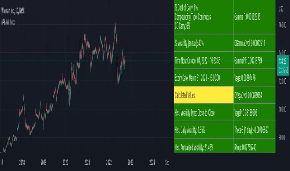
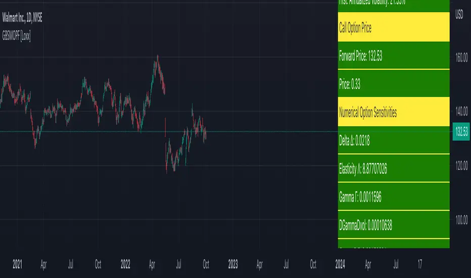
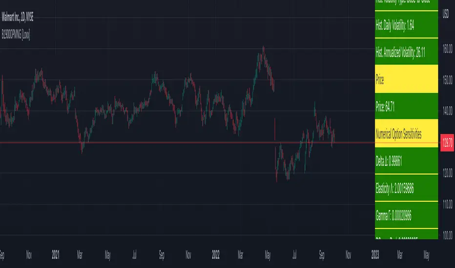
Black-Scholes 1973 OPM on Non-Dividend Paying Stocks [Loxx]Black-Scholes 1973 OPM on Non-Dividend Paying Stocks is an adaptation of the Black-Scholes-Merton Option Pricing Model including Analytical Greeks and implied volatility calculations. Making b equal to r yields the BSM model where dividends are not considered. The following information is an excerpt from Espen Gaarder Haug's book "Option Pricing Formulas". The options sensitivities (Greeks) are the partial derivatives of the Black-Scholes-Merton ( BSM ) formula. For our purposes here are, Analytical Greeks are broken down into various categories:
Delta Greeks: Delta, DDeltaDvol, Elasticity
Gamma Greeks: Gamma, GammaP, DGammaDSpot/speed, DGammaDvol/Zomma
Vega Greeks: Vega , DVegaDvol/Vomma, VegaP
Theta Greeks: Theta
Rate/Carry Greeks: Rho
Probability Greeks: StrikeDelta, Risk Neutral Density
(See the code for more details)
Black-Scholes-Merton Option Pricing
The BSM formula and its binomial counterpart may easily be the most used "probability model/tool" in everyday use — even if we con- sider all other scientific disciplines. Literally tens of thousands of people, including traders, market makers, and salespeople, use option formulas several times a day. Hardly any other area has seen such dramatic growth as the options and derivatives businesses. In this chapter we look at the various versions of the basic option formula. In 1997 Myron Scholes and Robert Merton were awarded the Nobel Prize (The Bank of Sweden Prize in Economic Sciences in Memory of Alfred Nobel). Unfortunately, Fischer Black died of cancer in 1995 before he also would have received the prize.
It is worth mentioning that it was not the option formula itself that Myron Scholes and Robert Merton were awarded the Nobel Prize for, the formula was actually already invented, but rather for the way they derived it — the replicating portfolio argument, continuous- time dynamic delta hedging, as well as making the formula consistent with the capital asset pricing model (CAPM). The continuous dynamic replication argument is unfortunately far from robust. The popularity among traders for using option formulas heavily relies on hedging options with options and on the top of this dynamic delta hedging, see Higgins (1902), Nelson (1904), Mello and Neuhaus (1998), Derman and Taleb (2005), as well as Haug (2006) for more details on this topic. In any case, this book is about option formulas and not so much about how to derive them.
Provided here are the various versions of the Black-Scholes-Merton formula presented in the literature. All formulas in this section are originally derived based on the underlying asset S follows a geometric Brownian motion
dS = mu * S * dt + v * S * dz
where t is the expected instantaneous rate of return on the underlying asset, a is the instantaneous volatility of the rate of return, and dz is a Wiener process.
The formula derived by Black and Scholes (1973) can be used to value a European option on a stock that does not pay dividends before the option's expiration date. Letting c and p denote the price of European call and put options, respectively, the formula states that
c = S * N(d1) - X * e^(-r * T) * N(d2)
p = X * e^(-r * T) * N(d2) - S * N(d1)
where
d1 = (log(S / X) + (r + v^2 / 2) * T) / (v * T^0.5)
d2 = (log(S / X) + (r - v^2 / 2) * T) / (v * T^0.5) = d1 - v * T^0.5
**This version of the Black-Scholes formula can also be used to price American call options on a non-dividend-paying stock, since it will never be optimal to exercise the option before expiration.**
Inputs
S = Stock price.
X = Strike price of option.
T = Time to expiration in years.
r = Risk-free rate
b = Cost of carry
v = Volatility of the underlying asset price
cnd (x) = The cumulative normal distribution function
nd(x) = The standard normal density function
convertingToCCRate(r, cmp ) = Rate compounder
gImpliedVolatilityNR(string CallPutFlag, float S, float x, float T, float r, float b, float cm , float epsilon) = Implied volatility via Newton Raphson
gBlackScholesImpVolBisection(string CallPutFlag, float S, float x, float T, float r, float b, float cm ) = implied volatility via bisection
Implied Volatility: The Bisection Method
The Newton-Raphson method requires knowledge of the partial derivative of the option pricing formula with respect to volatility ( vega ) when searching for the implied volatility . For some options (exotic and American options in particular), vega is not known analytically. The bisection method is an even simpler method to estimate implied volatility when vega is unknown. The bisection method requires two initial volatility estimates (seed values):
1. A "low" estimate of the implied volatility , al, corresponding to an option value, CL
2. A "high" volatility estimate, aH, corresponding to an option value, CH
The option market price, Cm , lies between CL and cH . The bisection estimate is given as the linear interpolation between the two estimates:
v(i + 1) = v(L) + (c(m) - c(L)) * (v(H) - v(L)) / (c(H) - c(L))
Replace v(L) with v(i + 1) if c(v(i + 1)) < c(m), or else replace v(H) with v(i + 1) if c(v(i + 1)) > c(m) until |c(m) - c(v(i + 1))| <= E, at which point v(i + 1) is the implied volatility and E is the desired degree of accuracy.
Implied Volatility: Newton-Raphson Method
The Newton-Raphson method is an efficient way to find the implied volatility of an option contract. It is nothing more than a simple iteration technique for solving one-dimensional nonlinear equations (any introductory textbook in calculus will offer an intuitive explanation). The method seldom uses more than two to three iterations before it converges to the implied volatility . Let
v(i + 1) = v(i) + (c(v(i)) - c(m)) / (dc / dv (i))
until |c(m) - c(v(i + 1))| <= E at which point v(i + 1) is the implied volatility , E is the desired degree of accuracy, c(m) is the market price of the option, and dc/ dv (i) is the vega of the option evaluaated at v(i) (the sensitivity of the option value for a small change in volatility ).
Things to know
Only works on the daily timeframe and for the current source price.
You can adjust the text size to fit the screen

Generalized Black-Scholes-Merton w/ Analytical Greeks [Loxx]Generalized Black-Scholes-Merton w/ Analytical Greeks is an adaptation of the Black-Scholes-Merton Option Pricing Model including Analytical Greeks and implied volatility calculations. The following information is an excerpt from Espen Gaarder Haug's book "Option Pricing Formulas". The options sensitivities (Greeks) are the partial derivatives of the Black-Scholes-Merton (BSM) formula. Analytical Greeks for our purposes here are broken down into various categories:
Delta Greeks: Delta, DDeltaDvol, Elasticity
Gamma Greeks: Gamma, GammaP, DGammaDSpot/speed, DGammaDvol/Zomma
Vega Greeks: Vega, DVegaDvol/Vomma, VegaP
Theta Greeks: Theta
Rate/Carry Greeks: Rho, Rho futures option, Carry Rho, Phi/Rho2
Probability Greeks: StrikeDelta, Risk Neutral Density
(See the code for more details)
Black-Scholes-Merton Option Pricing
The BSM formula and its binomial counterpart may easily be the most used "probability model/tool" in everyday use — even if we con- sider all other scientific disciplines. Literally tens of thousands of people, including traders, market makers, and salespeople, use option formulas several times a day. Hardly any other area has seen such dramatic growth as the options and derivatives businesses. In this chapter we look at the various versions of the basic option formula. In 1997 Myron Scholes and Robert Merton were awarded the Nobel Prize (The Bank of Sweden Prize in Economic Sciences in Memory of Alfred Nobel). Unfortunately, Fischer Black died of cancer in 1995 before he also would have received the prize.
It is worth mentioning that it was not the option formula itself that Myron Scholes and Robert Merton were awarded the Nobel Prize for, the formula was actually already invented, but rather for the way they derived it — the replicating portfolio argument, continuous- time dynamic delta hedging, as well as making the formula consistent with the capital asset pricing model (CAPM). The continuous dynamic replication argument is unfortunately far from robust. The popularity among traders for using option formulas heavily relies on hedging options with options and on the top of this dynamic delta hedging, see Higgins (1902), Nelson (1904), Mello and Neuhaus (1998), Derman and Taleb (2005), as well as Haug (2006) for more details on this topic. In any case, this book is about option formulas and not so much about how to derive them.
Provided here are the various versions of the Black-Scholes-Merton formula presented in the literature. All formulas in this section are originally derived based on the underlying asset S follows a geometric Brownian motion
dS = mu * S * dt + v * S * dz
where t is the expected instantaneous rate of return on the underlying asset, a is the instantaneous volatility of the rate of return, and dz is a Wiener process.
The formula derived by Black and Scholes (1973) can be used to value a European option on a stock that does not pay dividends before the option's expiration date. Letting c and p denote the price of European call and put options, respectively, the formula states that
c = S * N(d1) - X * e^(-r * T) * N(d2)
p = X * e^(-r * T) * N(d2) - S * N(d1)
where
d1 = (log(S / X) + (r + v^2 / 2) * T) / (v * T^0.5)
d2 = (log(S / X) + (r - v^2 / 2) * T) / (v * T^0.5) = d1 - v * T^0.5
Inputs
S = Stock price.
X = Strike price of option.
T = Time to expiration in years.
r = Risk-free rate
b = Cost of carry
v = Volatility of the underlying asset price
cnd (x) = The cumulative normal distribution function
nd(x) = The standard normal density function
convertingToCCRate(r, cmp ) = Rate compounder
gImpliedVolatilityNR(string CallPutFlag, float S, float x, float T, float r, float b, float cm , float epsilon) = Implied volatility via Newton Raphson
gBlackScholesImpVolBisection(string CallPutFlag, float S, float x, float T, float r, float b, float cm ) = implied volatility via bisection
Implied Volatility: The Bisection Method
The Newton-Raphson method requires knowledge of the partial derivative of the option pricing formula with respect to volatility ( vega ) when searching for the implied volatility . For some options (exotic and American options in particular), vega is not known analytically. The bisection method is an even simpler method to estimate implied volatility when vega is unknown. The bisection method requires two initial volatility estimates (seed values):
1. A "low" estimate of the implied volatility , al, corresponding to an option value, CL
2. A "high" volatility estimate, aH, corresponding to an option value, CH
The option market price, Cm , lies between CL and cH . The bisection estimate is given as the linear interpolation between the two estimates:
v(i + 1) = v(L) + (c(m) - c(L)) * (v(H) - v(L)) / (c(H) - c(L))
Replace v(L) with v(i + 1) if c(v(i + 1)) < c(m), or else replace v(H) with v(i + 1) if c(v(i + 1)) > c(m) until |c(m) - c(v(i + 1))| <= E, at which point v(i + 1) is the implied volatility and E is the desired degree of accuracy.
Implied Volatility: Newton-Raphson Method
The Newton-Raphson method is an efficient way to find the implied volatility of an option contract. It is nothing more than a simple iteration technique for solving one-dimensional nonlinear equations (any introductory textbook in calculus will offer an intuitive explanation). The method seldom uses more than two to three iterations before it converges to the implied volatility . Let
v(i + 1) = v(i) + (c(v(i)) - c(m)) / (dc / dv (i))
until |c(m) - c(v(i + 1))| <= E at which point v(i + 1) is the implied volatility , E is the desired degree of accuracy, c(m) is the market price of the option, and dc/ dv (i) is the vega of the option evaluaated at v(i) (the sensitivity of the option value for a small change in volatility ).
Things to know
Only works on the daily timeframe and for the current source price.
You can adjust the text size to fit the screen

Generalized Black-Scholes-Merton Option Pricing Formula [Loxx]Generalized Black-Scholes-Merton Option Pricing Formula is an adaptation of the Black-Scholes-Merton Option Pricing Model including Numerical Greeks aka "Option Sensitivities" and implied volatility calculations. The following information is an excerpt from Espen Gaarder Haug's book "Option Pricing Formulas".
Black-Scholes-Merton Option Pricing
The BSM formula and its binomial counterpart may easily be the most used "probability model/tool" in everyday use — even if we con- sider all other scientific disciplines. Literally tens of thousands of people, including traders, market makers, and salespeople, use option formulas several times a day. Hardly any other area has seen such dramatic growth as the options and derivatives businesses. In this chapter we look at the various versions of the basic option formula. In 1997 Myron Scholes and Robert Merton were awarded the Nobel Prize (The Bank of Sweden Prize in Economic Sciences in Memory of Alfred Nobel). Unfortunately, Fischer Black died of cancer in 1995 before he also would have received the prize.
It is worth mentioning that it was not the option formula itself that Myron Scholes and Robert Merton were awarded the Nobel Prize for, the formula was actually already invented, but rather for the way they derived it — the replicating portfolio argument, continuous- time dynamic delta hedging, as well as making the formula consistent with the capital asset pricing model (CAPM). The continuous dynamic replication argument is unfortunately far from robust. The popularity among traders for using option formulas heavily relies on hedging options with options and on the top of this dynamic delta hedging, see Higgins (1902), Nelson (1904), Mello and Neuhaus (1998), Derman and Taleb (2005), as well as Haug (2006) for more details on this topic. In any case, this book is about option formulas and not so much about how to derive them.
Provided here are the various versions of the Black-Scholes-Merton formula presented in the literature. All formulas in this section are originally derived based on the underlying asset S follows a geometric Brownian motion
dS = mu * S * dt + v * S * dz
where t is the expected instantaneous rate of return on the underlying asset, a is the instantaneous volatility of the rate of return, and dz is a Wiener process.
The formula derived by Black and Scholes (1973) can be used to value a European option on a stock that does not pay dividends before the option's expiration date. Letting c and p denote the price of European call and put options, respectively, the formula states that
c = S * N(d1) - X * e^(-r * T) * N(d2)
p = X * e^(-r * T) * N(d2) - S * N(d1)
where
d1 = (log(S / X) + (r + v^2 / 2) * T) / (v * T^0.5)
d2 = (log(S / X) + (r - v^2 / 2) * T) / (v * T^0.5) = d1 - v * T^0.5
Inputs
S = Stock price.
X = Strike price of option.
T = Time to expiration in years.
r = Risk-free rate
b = Cost of carry
v = Volatility of the underlying asset price
cnd (x) = The cumulative normal distribution function
nd(x) = The standard normal density function
convertingToCCRate(r, cmp ) = Rate compounder
gImpliedVolatilityNR(string CallPutFlag, float S, float x, float T, float r, float b, float cm, float epsilon) = Implied volatility via Newton Raphson
gBlackScholesImpVolBisection(string CallPutFlag, float S, float x, float T, float r, float b, float cm) = implied volatility via bisection
Implied Volatility: The Bisection Method
The Newton-Raphson method requires knowledge of the partial derivative of the option pricing formula with respect to volatility (vega) when searching for the implied volatility. For some options (exotic and American options in particular), vega is not known analytically. The bisection method is an even simpler method to estimate implied volatility when vega is unknown. The bisection method requires two initial volatility estimates (seed values):
1. A "low" estimate of the implied volatility, al, corresponding to an option value, CL
2. A "high" volatility estimate, aH, corresponding to an option value, CH
The option market price, Cm, lies between CL and cH. The bisection estimate is given as the linear interpolation between the two estimates:
v(i + 1) = v(L) + (c(m) - c(L)) * (v(H) - v(L)) / (c(H) - c(L))
Replace v(L) with v(i + 1) if c(v(i + 1)) < c(m), or else replace v(H) with v(i + 1) if c(v(i + 1)) > c(m) until |c(m) - c(v(i + 1))| <= E, at which point v(i + 1) is the implied volatility and E is the desired degree of accuracy.
Implied Volatility: Newton-Raphson Method
The Newton-Raphson method is an efficient way to find the implied volatility of an option contract. It is nothing more than a simple iteration technique for solving one-dimensional nonlinear equations (any introductory textbook in calculus will offer an intuitive explanation). The method seldom uses more than two to three iterations before it converges to the implied volatility. Let
v(i + 1) = v(i) + (c(v(i)) - c(m)) / (dc / dv(i))
until |c(m) - c(v(i + 1))| <= E at which point v(i + 1) is the implied volatility, E is the desired degree of accuracy, c(m) is the market price of the option, and dc/dv(i) is the vega of the option evaluaated at v(i) (the sensitivity of the option value for a small change in volatility).
Numerical Greeks or Greeks by Finite Difference
Analytical Greeks are the standard approach to estimating Delta, Gamma etc... That is what we typically use when we can derive from closed form solutions. Normally, these are well-defined and available in text books. Previously, we relied on closed form solutions for the call or put formulae differentiated with respect to the Black Scholes parameters. When Greeks formulae are difficult to develop or tease out, we can alternatively employ numerical Greeks - sometimes referred to finite difference approximations. A key advantage of numerical Greeks relates to their estimation independent of deriving mathematical Greeks. This could be important when we examine American options where there may not technically exist an exact closed form solution that is straightforward to work with. (via VinegarHill FinanceLabs)
Things to know
Only works on the daily timeframe and for the current source price.
You can adjust the text size to fit the screen
Bachelier 1900 Option Pricing Model w/ Numerical Greeks [Loxx]Bachelier 1900 Option Pricing Model w/ Numerical Greeks is an adaptation of the Bachelier 1900 Option Pricing Model in Pine Script. The following information is an except from Espen Gaarder Haug's book "Option Pricing Formulas"
Before Black Scholes Merton
The curious reader may be asking how people priced options before the BSM breakthrough was published in 1973. This section offers a quick overview of some of the most important precursors to the BSM model. As early as 1900, Louis Bachelier published his now famous work on option pricing. In contrast to Black, Scholes, and Merton, Bachelier assumed a normal distribution for the asset price—in other words, an arithmetic Brownian motion process:
dS = sigma * dz
Where S is the asset price and dz is a Wiener process. This implies a positive probability for observing a negative asset price—a feature that is not popular for stocks and any other asset with limited liability features.
The current call price is the expected price at expiration. This argument yields:
c = (S - X)*N(d1) + v * T^0.5 * n(d1)
and for a put option we get
p = (S - X)*N(-d1) + v * T^0.5 * n(d1)
where
d1 = (S - X) / (v * T^0.5)
Inputs
S = Stock price.
X = Strike price of option.
T = Time to expiration in years.
v = Volatility of the underlying asset price
cnd(x) = The cumulative normal distribution function
nd(x) = The standard normal density function
Numerical Greeks or Greeks by Finite Difference
Analytical Greeks are the standard approach to estimating Delta, Gamma etc... That is what we typically use when we can derive from closed form solutions. Normally, these are well-defined and available in text books. Previously, we relied on closed form solutions for the call or put formulae differentiated with respect to the Black Scholes parameters. When Greeks formulae are difficult to develop or tease out, we can alternatively employ numerical Greeks - sometimes referred to finite difference approximations. A key advantage of numerical Greeks relates to their estimation independent of deriving mathematical Greeks. This could be important when we examine American options where there may not technically exist an exact closed form solution that is straightforward to work with. ( via VinegarHill FinanceLabs )
Things to know
Volatility for this model is price, so dollars or whatever currency you're using. Historical volatility is also reported in currency.
There is no risk-free rate input
There is no dividend adjustment input
RSI Average Swing BotThis is a modified RSI version using as a source a big length(50 candles) and an average of all types of sources for candle calculations such as ohlc4, close, high, open, hlc3 and hl2.
In this case we are going to use a 0-1 scale for an easier calculation, where 0.5 is going to be our middle point.
Above 0.5 we consider a bullish possibility.
Below 0.5 we consider a bearish possibility.
I made a small example bot using that initial logic, together with 2 exit points for long or short positions.
If there are any questions, let me know !

quantized pin bar indicator with ATRAbstract
This script computes the strength of pin bars.
This script uses the corrent and the previous two bars to compute the strength of pin bars.
The strength of pin bars can be also comared with average true range, so we can evaluate those pin bars are strong or weak.
Introduction
Pin bar is a popular price action trading strategy.
It is based on quick price rejection.
Most of existing pin bar scripts only determine if a bar is a pin bar or not.
However, evaluating the strength of pin bars is important.
If price rejection is too weak, it is difficult to trigger trend reversal.
If a pin bar is too strong, we may enter the trade too late and cannot have good profit.
In this script, it provides a method to compute to strength of pin bars.
After the strength of pin bars are quantized, they can compare with average true range, price range and trend strength, which can help us to determine where are worthy for us to open trades.
Computation
Bullish hammer : current low is lower than ( previous high or current open ) and current close.
Bearish gravestone : current high is higher than ( previous low or current open ) and current close.
Bullish engulfing and harami : ( current low or previous low ) is lower than ( previous 2nd high or previous open ) and current close.
Bearish engulfing and harami : ( current high or previous high ) is higher than ( previous 2nd low or previous open ) and current close.
Parameters
Smoothing : the type of computing average.
Length of ATR : determines the number of true ranges for computing average true range.
ATR multiplier line : the threshould that a pin bar is strong enough. For example, if this value is 0.5, it means a pin bar with 0.5*atr or more is considered a strong pin bar.
one direction pinbar : set to 1 if you want the strength of bullish pin bars and bearish pin bars are cancelled. Set to 0 if you want to keep both strength of bullish pin bars and bearish pin bars; in this case, you may need to change the plot style to make both strength visible.
Trading Suggestions
Evaluate the strength of trend against pin bars. After all, a single reverse pin bar may be too weak to reverse the trend.
Timeframe : if atr is higher than 4*spread, the timeframe is high enough. However, if strong pin bars appear too frequent or price range is too small, going to higher fimeframe may be more safe.
Entry and exit : according to personal flavors.
Conclusion
The strength of pin bars can be quantized.
With this indicator, we can find more potential pin bars which human eyes and binary pattern detectors were leaked.
In my opinion, 0.5*atr is the most suitable streng of a pin bar for my trade entry but I still need to consider the direction of the trend.
You are welcome to share your settings and related trading strategy.
References
Most of related knowledge can be searched from the internet.
I cannot say the exact references because they may violate the rules of Tradingview.

Neglected Volume by DGTVolume is one piece of information that is often neglected, however, learning to interpret volume brings many advantages and could be of tremendous help when it comes to analyzing the markets. In addition to technicians, fundamental investors also take notice of the numbers of shares traded for a given security.
What is Volume?
The volume represents all the recorded trades for a security that occurs in a given time interval. It is a measurement of the participation, enthusiasm, and interest in a given security. Think of volume as the force that drives the market. Volume substantiates, energizes, and empowers price. When volume increases, it confirms price direction; when volume decreases, it contradicts price direction.
In theory, increases in volume generally precede significant price movements. However, If the price is rising in an uptrend but the volume is reducing or unchanged, it may show that there’s little interest in the security, and the price may reverse.
A high volume usually indicates more interest in the security and the presence of institutional traders. However, a rapidly rising price in an uptrend accompanied by a huge volume may be a sign of exhaustion.
Traders usually look for breaks of support and resistance to enter positions. When security break critical levels without volume, you should consider the breakout suspect and prime for a reversal off the highs/lows
Volume spikes are often the result of news-driven events. Volume spike will often lead to sharp reversals since the moves are unsustainable due to the imbalance of supply and demand
note : there’s no centralized exchange where trades are recorded, so the volume data represents what happens at a particular exchange only
In most charting platforms, the volume indicator is presented as color-coded bars, green if the security closes up and red if the security closed lower, where the height of the bars show the amount of the recorded trades
Within this study, Relative Volume , Volume Weighted Bars and Volume Moving Average are presented, where Relative Volume relates current trading volume to past trading volume over long period, Volume Weighted Bars presents price bars colored based on short period past trading volume average, and Volume Moving Average is average of volume over shot period
Relative Volume is presented as color-coded bars similar to regular Volume indicator but uses four color codes instead two. Notable increases of volume are presented in green and red while average values with back and gray, hence adding ability to emphasis notable increases in the volume. It is kind of a like a radar for how "in-play" a security is. Users are allowed to change the threshold, default value is set to Fibonacci golden ration standard deviation away from its moving average.
Volume Weighted Bars, a study of Kıvanç Özbilgiç, aims to present if price movements are supported by Volume. Volume Weighted Bars are calculated based on shot period volume moving average which will reflect more recent changes in volume. Price actions with high volume will be displayed with darker colors, average volume values will remain as they are and low volume values will be indicated with lighter colors.
Volume Moving Average, Is short period volume moving average, aims to display visually the volume changes. Please not that Relative Volume bars are calculated based on standard deviation of long volume moving average.
What Else?
Apart from the volume itself, your ability to assess what volume is telling you in conjunction with price action can be a key factor in your ability to turn a profit in the market. It makes little sense to analyze the volume alone. To correctly interpret the volume data, it shall be seen in the light of what the price is doing. there are a lot of other indicators that are based on the volume data as well as price action. Analysing those volume indicators has always helped traders and investors to better understand what is happening in the market.
Here are the ones adapted with this study. Some of them used as a source for our aim, some adapted as they are with slight changes to fit visually to this study and please note that the numerical presentation may differ from their regular use
• On Balance Volume
• Divergence Indicator
• Correlation Coefficient
• Chaikin Money Flow
Shortly;
On Balance Volume
The On Balance Volume indicator, is a technical analysis indicator that relates volume flow to changes in a security’s price. It uses a cumulative total of positive and negative trading volume to predict the direction of price. The OBV is a volume-based momentum oscillator, so it is a leading indicator — it changes direction before the price
Granville, creator of OBV, proposed the theory that changes in volume precede price movements in a measurable way. He believed that volume was the main force behind major market moves and thought of OBV’s prediction of price changes as a compressed spring that expands rapidly when released.
It is believed that the OBV shows the interactions between the institutional and retail traders in the market
If the price makes a new high, the OBV should also make a new high. If the OBV makes a lower high when the price makes a higher high, there’s a classical bearish divergence — indicating that only the retail traders are buying. Another type of bearish divergence occurs when the price remains relatively quiet and fails to make a higher high but the OBV soars higher than the previous high — indicating that the institutional traders are accumulating short positions. On the other hand, if the price makes a lower low and the OBV makes a higher low, there is a classical bullish divergence, showing that the institutional traders don’t believe in that move
With this study, Momentum and Acceleration (optional) of OBV is calculated and presented, where momentum is most commonly referred to as a rate and measures the acceleration of the price and/or volume of a security. It is also referred to as a technical analysis indicator and oscillator that is able to determine market trends.
Additionally, smoothing functionality with Least Squares Method is added
Divergences especially, should always be noted as a possible reversal in the current trend, so the divergence indicator is adapted with this study where the Momentum of OBV is assumed as Oscillator with similar usages as to RSI. Divergence is most often used to track and analyze the momentum in an asset’s price and the odds of a price reversal within the current trend. The divergence indicator warns traders and technical analysts of changes in a price/volume trend, oftentimes that it is weakening or changing direction.
Correlation Coefficient
The correlation coefficient is a statistical measure of the strength of the relationship between the relative movements of two variables. A correlation of -1.0 shows a perfect negative correlation, while a correlation of 1.0 shows a perfect positive correlation. A correlation of 0.0 shows no linear relationship between the movement of the two variables. In other words, the closer the Correlation Coefficient is to 1.0, indicates the instruments will move up and down together as it is mostly expected with volume and price. So the Correlation Coefficient Indicator aims to display when the price and volume (on balance volume) is in correlation and when not. With this study blue represent positive correlation while orange negative correlation. The strength of the correlation is determined by the width of the bands, to emphasis the effect horizontal lines are drawn with values set to 0.5 and -0.5. the values above 0.5 (or below -0.5) shows stronger correlation.
Chaikin Money Flow , provide optionally as a companion indicator
The Chaikin money flow indicator (CMF) is a volume indicator that measures the money flow volume over a chosen period. The money flow volume is a measure of the volume and where the price closed relative to the trading session’s range. It comes from the idea that buying pressure is indicated by a rising volume and recurrent closes in the upper part of the session’s price range while selling pressure is demonstrated by an increasing volume and repeated closes in the lower part of the price range.
Both buying and selling pressures are accompanied by an increase in volume, but the location of the closing prices are in accordance with the direction of price
Special thanks to @InvestCHK and @hjsjshs , who have enormously contributed while preparing this study
related studies:
Disclaimer:
Trading success is all about following your trading strategy and the indicators should fit within your trading strategy, and not to be traded upon solely
The script is for informational and educational purposes only. Use of the script does not constitute professional and/or financial advice. You alone have the sole responsibility of evaluating the script output and risks associated with the use of the script. In exchange for using the script, you agree not to hold dgtrd TradingView user liable for any possible claim for damages arising from any decision you make based on use of the script

Filter Information Box - PineCoders FAQWhen designing filters it can be interesting to have information about their characteristics, which can be obtained from the set of filter coefficients (weights). The following script analyzes the impulse response of a filter in order to return the following information:
Lag
Smoothness via the Herfindahl index
Percentage Overshoot
Percentage Of Positive Weights
The script also attempts to determine the type of the analyzed filter, and will issue warnings when the filter shows signs of unwanted behavior.
DISPLAYED INFORMATION AND METHODS
The script displays one box on the chart containing two sections. The filter metrics section displays the following information:
- Lag : Measured in bars and calculated from the convolution between the filter's impulse response and a linearly increasing sequence of value 0,1,2,3... . This sequence resets when the impulse response crosses under/over 0.
- Herfindahl index : A measure of the filter's smoothness described by Valeriy Zakamulin. The Herfindahl index measures the concentration of the filter weights by summing the squared filter weights, with lower values suggesting a smoother filter. With normalized weights the minimum value of the Herfindahl index for low-pass filters is 1/N where N is the filter length.
- Percentage Overshoot : Defined as the maximum value of the filter step response, minus 1 multiplied by 100. Larger values suggest higher overshoots.
- Percentage Positive Weights : Percentage of filter weights greater than 0.
Each of these calculations is based on the filter's impulse response, with the impulse position controlled by the Impulse Position setting (its default is 1000). Make sure the number of inputs the filter uses is smaller than Impulse Position and that the number of bars on the chart is also greater than Impulse Position . In order for these metrics to be as accurate as possible, make sure the filter weights add up to 1 for low-pass and band-stop filters, and 0 for high-pass and band-pass filters.
The comments section displays information related to the type of filter analyzed. The detection algorithm is based on the metrics described above. The script can detect the following type of filters:
All-Pass
Low-Pass
High-Pass
Band-Pass
Band-Stop
It is assumed that the user is analyzing one of these types of filters. The comments box also displays various warnings. For example, a warning will be displayed when a low-pass/band-stop filter has a non-unity pass-band, and another is displayed if the filter overshoot is considered too important.
HOW TO SET THE SCRIPT UP
In order to use this script, the user must first enter the filter settings in the section provided for this purpose in the top section of the script. The filter to be analyzed must then be entered into the:
f(input)
function, where `input` is the filter's input source. By default, this function is a simple moving average of period length . Be sure to remove it.
If, for example, we wanted to analyze a Blackman filter, we would enter the following:
f(input)=>
pi = 3.14159,sum = 0.,sumw = 0.
for i = 0 to length-1
k = i/length
w = 0.42 - 0.5 * cos(2 * pi * k) + 0.08 * cos(4 * pi * k)
sumw := sumw + w
sum := sum + w*input
sum/sumw
EXAMPLES
In this section we will look at the information given by the script using various filters. The first filter we will showcase is the linearly weighted moving average (WMA) of period 9.
As we can see, its lag is 2.6667, which is indeed correct as the closed form of the lag of the WMA is equal to (period-1)/3 , which for period 9 gives (9-1)/3 which is approximately equal to 2.6667. The WMA does not have overshoots, this is shown by the the percentage overshoot value being equal to 0%. Finally, the percentage of positive weights is 100%, as the WMA does not possess negative weights.
Lets now analyze the Hull moving average of period 9. This moving average aims to provide a low-lag response.
Here we can see how the lag is way lower than that of the WMA. We can also see that the Herfindahl index is higher which indicates the WMA is smoother than the HMA. In order to reduce lag the HMA use negative weights, here 55% (as there are 45% of positive ones). The use of negative weights creates overshoots, we can see with the percentage overshoot being 26.6667%.
The WMA and HMA are both low-pass filters. In both cases the script correctly detected this information. Let's now analyze a simple high-pass filter, calculated as follows:
input - sma(input,length)
Most weights of a high-pass filters are negative, which is why the lag value is negative. This would suggest the indicator is able to predict future input values, which of course is not possible. In the case of high-pass filters, the Herfindahl index is greater than 0.5 and converges toward 1, with higher values of length . The comment box correctly detected the type of filter we were using.
Let's now test the script using the simple center of gravity bandpass filter calculated as follows:
wma(input,length) - sma(input,length)
The script correctly detected the type of filter we are using. Another type of filter that the script can detect is band-stop filters. A simple band-stop filter can be made as follows:
input - (wma(input,length) - sma(input,length))
The script correctly detect the type of filter. Like high-pass filters the Herfindahl index is greater than 0.5 and converges toward 1, with greater values of length . Finally the script can detect all-pass filters, which are filters that do not change the frequency content of the input.
WARNING COMMENTS
The script can give warning when certain filter characteristics are detected. One of them is non-unity pass-band for low-pass filters. This warning comment is displayed when the weights of the filter do not add up to 1. As an example, let's use the following function as a filter:
sum(input,length)
Here the filter pass-band has non unity, and the sum of the weights is equal to length . Therefore the script would display the following comments:
We can also see how the metrics go wild (note that no filter type is detected, as the detected filter could be of the wrong type). The comment mentioning the detection of high overshoot appears when the percentage overshoot is greater than 50%. For example if we use the following filter:
5*wma(input,length) - 4*sma(input,length)
The script would display the following comment:
We can indeed see high overshoots from the filter:
@alexgrover for PineCoders
Look first. Then leap.

Filter Amplitude Response Estimator - A Simple CalculationIn digital signal processing knowing how a system interact with the frequency content of an input signal is extremely important, the mathematical tool that give you this information is called "frequency response". The frequency response regroup two elements, the amplitude response, and the phase response. The amplitude response tells you how the system modify the amplitude of the frequency components in the input signal, the phase response tells you how the system modify the phase of the frequency components in the signal, each being a function of the frequency.
The today proposed tool aim to give a low resolution representation of the amplitude response of any filter.
What Is The Amplitude Response Of A Filter ?
Remember that filters allow to interact with the frequency content of a signal by amplifying, attenuating and/or removing certain frequency components in the input signal, the amplitude (also called magnitude) response of a filter let you know exactly how your filter change the amplitude of the frequency components in the input signal, another way to see the amplitude response is as a tool that tell you what is the peak amplitude of a filter using a sinusoid of a certain frequency as input signal.
For example if the amplitude response of a filter give you a value of 0.9 at frequency 0.5, it means that the filter peak amplitude using a sinusoid of frequency 0.5 is equal to 0.9.
There are several ways to calculate the frequency response of a filter, when our filter is a FIR filter (the filter impulse response is finite), the frequency response of the filter is the absolute value of the discrete Fourier transform (DFT) of the filter impulse response.
If you are curious about this process, know that the DFT of a N samples signal return N values, so if our FIR filter coefficients are composed of only 5 values we would get a frequency response of 5 values...which would not be useful, this is why we "pad" our coefficients with zeros, that is we add zeros to the start and end of our series of coefficients, this process is called "zero-padding", so if our series of coefficients is: (1,2,3,4,5), applying zero padding would give (0,0...1,2,3,4,5,...0,0) while keeping a certain symmetry. This is related to the concept of resolution, a low resolution amplitude response would be composed of a low number of values and would not be useful, this is why we use zero-padding to add more values thus increasing the resolution.
Making a Fourier transform in Pinescript is not doable, as you need the complex number i for computing a DFT, but thats not even the only problem, a DFT would not be that useful anyway (as the processes to make it useful in a trading context would be way too complex) . So how can we calculate a filter amplitude response without using a DFT ? The simple answer is by taking the peak amplitude of a filter using a sinusoid of a certain frequency as input, this is what the proposed tool do.
Using The Tool
The proposed tool give you a 50 point amplitude response from frequency 0.005 to 0.25 by default. the setting "Range Divisor" allow you to see the amplitude response by using a different range of frequency, for example if the range divisor is equal to 2 the filter amplitude response will be evaluated from frequency 0.0025 to 0.125.
In the script, filt hold the filter you want to see the frequency response, by default a simple moving average.
The position of the frequency response is defined by the "Show Amplitude Response At Bar Number" setting, if you want the frequency response to start at bar number 5000 then enter 5000, by default 10000. If you are not a premium set the number at 4000 and it should work.
amplitude response of a simple moving average of period 14, res = 2.
By default the amplitude response use an amplitude scale, a value of 1 represent an unchanged amplitude. You can use Dbfs (decibel full scale) instead by checking the "To Decibels (Full Scale)" setting.
Dbfs amplitude response, a value of 0 represent an unchanged amplitude.
Some Amplitude Responses
In order to prove the accuracy of the proposed tool we can compare the amplitude response given by the proposed tool with the mathematical function of the amplitude response of a simple moving average, that is:
abs(sin(pi*f*length)/(length*sin(pi*f)))
In cyan the amplitude response given by the proposed tool and in blue the above function. Below are the amplitude responses of some moving averages with period 14.
Amplitude response of an EMA, the EMA is a IIR filter, therefore the amplitude response can't be made by taking the DFT of the impulse response (as this ones has infinite length), however our tool can give its frequency response.
Amplitude response of the Hull MA, as you can see some frequencies are amplified, this is common with low-lag filters.
Gaussian moving average (ALMA), with offset = 0.5 and sigma = 6.
Simple moving average high-pass filter amplitude response
Center of gravity bandpass filter amplitude response
Center of gravity bandreject filter.
IMPORTANT!: The amplitude response of adaptive moving averages is not stationary and might change over time.
Conclusion
A tool giving the amplitude response of any filter has been presented, of course this method is not efficient at all and has a low resolution of 50 points (the common resolution is of 512 points) and is difficult to work with, but has the merit to work on Tradingview and can give the frequency response of IIR filters, if you really need to see the frequency response of a filter then i recommend you to use the function freqz from the scipy package.
I still hope you will enjoy using this tool to have a look at the amplitude responses of your favorite moving averages.
I'am aware of the current situation, however i'am somehow feeling left out from the pinescript community, let me know via PM if i have done something to you and i'll do my best to fix any problems i might have caused (or i might be being parano xD)

Multi-TF Avg BBandsMULTI-TF AVERAGE BBANDS - with signals (BETA)
Overall, it shows where the price has support and resistance, when it's breaking through, and when its relatively low/high based on the magic of standard deviation.
created by gamazama. send me a shout if u find this useful, or if you create something cool with it.
%BB: The price's position in the boilinger band is converted to a range from 0-1. The midpoint is at 0.5
Description of parameters
"BB:Window Length" is the standard BB size of 20 candles.
The indicator plots up to 7 different %BB's on different timescales
They are calculated independently of the timescale you are viewing eg 12h, 3d, 30m will be the same output
You can enter 7 timescales, eg. if you want to plot a range of bbands of the 12h up to 3d graphs, enter values between 0.5 and 3 (days) - you can also select 0 to disable and use less timescales, or select hours or minutes
Take note if you eg. double the main multiplier to 40, it is the same as doubling all your timescales
You can turn the transparency of the 7 x %BB's to 100 to hide them, their average is plotted as a thick cyan line
"Variance" is a measure of how much the 7 BB's agree, and changes colour based on the thresholds used for the strategy
---- TO START FROM SCRATCH ----
- set all except one to ZERO (0), set to 0, and everything after to 0.
Turn ON and right click -> move the indicator to a new pane - this will show you the internal workings of the indicator.
Then there is a few standard settings
"Source Smoothing Amount" applies a basic small sma on the price.
It should be turned down when viewing candles with less information, like 1D or more.
Standard BBands use an SMA, there one uses a blend between VWMA or SMA
Volume Weight settings, the same as SMA at 0, and the same as VWMA at 1
BB^2 is a bband drawn around the average %BB. Adjust the to change its window length
The BB^2 changes color when price moves up or down
Now its time to look at the parameters which affect the buy/sell signals
turn on "show signal range" - you see some red lines
buy and sell each have 4 settings
min/max variance will affect the brigtness of the signal range
range adjust will move the range up/down
mix BB^2 blends between a straight line (0) and BB^2's top or bottom (1)
a threshold of "variance" and "h/l points" is available to generate weaker signals.
these thresholds can be increased to show more weak signals
ONCE YOU ARE HAPPY WITH THE SIGNALS being generated, you can turn OFF , and move it back to the price pane
the indicator then draws a bband around the price to maps some info into the chart:
fills a colour between 0.5 & the mid BB^2 and converts relative to the price chart
draws a line in the middle of the midband.
controls how much these lines diverge from the price - adjust it to reduce noise
converts the signal range (red lines) to be relative to the price chart
if you like, you can adjust the sell & buy signals in the tab from and to and to match the picture. It messes with auto-scaling when moving back to though
enjoy, I hope that is easy enough to understand, still trying to make this more user-friendly.
If you want to send me some token of appreciation - btc: 33c2oiCW8Fnsy41Y8z2jAPzY8trnqr5cFu
I promise it will put a fat smile on my face
Closed Form Distance VolatilityIntroduction
Calculating distances in signal processing/statistics/time-series analysis imply measuring the distance between two probability distribution, i am not really familiar with distances but since some formulas are in closed form they can be easily used for volatility estimation. This volatility indicator will use three methods originally made to measure the distance of gaussian copulas, using those methods for volatility estimation is fairly easy and provide a different approach to statistical dispersion.
The indicator have a length parameter and a method parameter to select the method used for volatility estimation, i describe each methods below.
Hellinger Method
Each method will use the rolling sum of the low price and the rolling sum of the high price instead of probability distributions. The Hellinger method have many application from the measurement of distances to the use as a cost function for neural networks.
Its closed form is defined as the square root of 1 - a^0.25b^0.25/(0.5a + 0.5b)^0.5 where a and b are both positive series. In our indicator a is the rolling sum of the high price and b the rolling sum of the low price. This method give a classic estimation of volatility.
Bhattacharyya Method
The Bhattacharyya method is another method who use a natural logarithm, this method can visually filter small volatility variation. It is defined as 0.5 * log((0.5a+0.5b)/√(ab)) .
Wasserstein Method
This method was originally using a trimmed mean for its calculation. The original method is defined as the square of the trimmed mean of a + b - 2√(a^0.5ba^0.5) , a median has been used instead of a trimmed mean for efficiency sake, both central tendency estimators are robust to outliers.
Conclusion
I showed that closed form formulas for distance calculation could be derived into volatility estimators with different properties. They could be used with series in a range of (0,1) to provide a smoothing variable for exponential smoothing.

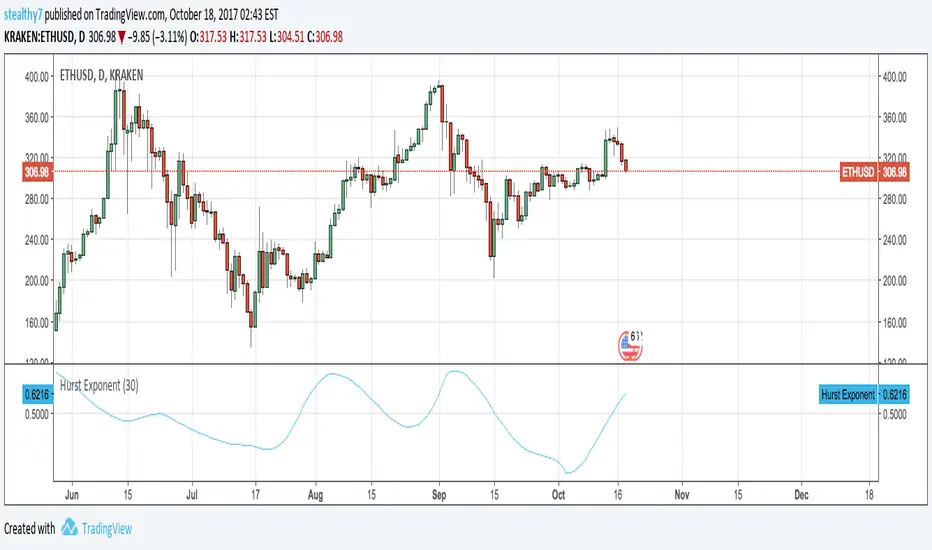
Stealthy Hurst ExponentThis is my attempt at Hurst Exponent indicator.
Above 0.5 is supposed to indicate a trend is present.
Below 0.5 is noise.
0.5 is supposed to be Brownian Motion or regular market noise.
If you have corrections to the code you want to share, please post it.
I'm not an expert in math or coding, so this shouldn't be copied / ported.
This code didn't work very well as a filter, but you may have a fix or other use.
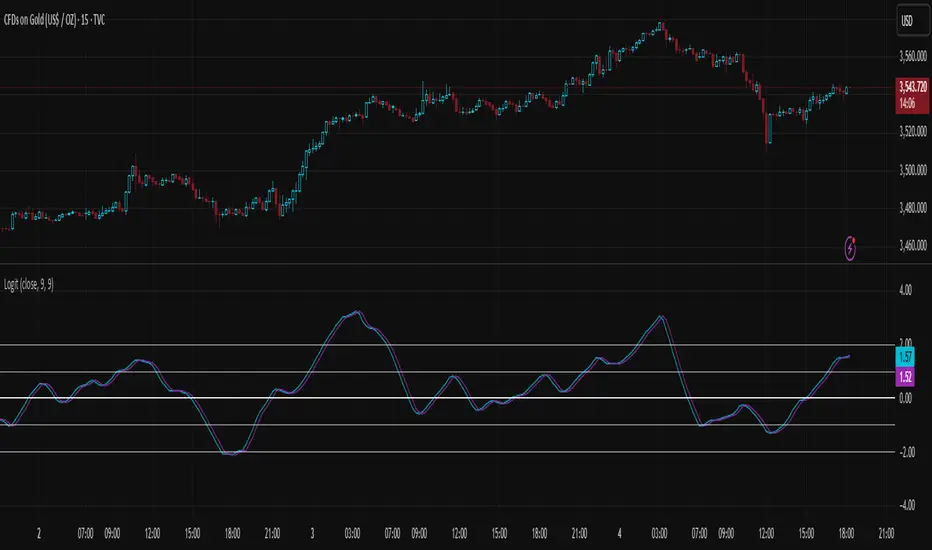
Logit Transform -EasyNeuro-Logit Transform
This script implements a novel indicator inspired by the Fisher Transform, replacing its core arctanh-based mapping with the logit transform. It is designed to highlight extreme values in bounded inputs from a probabilistic and statistical perspective.
Background: Fisher Transform
The Fisher Transform, introduced by John Ehlers , is a statistical technique that maps a bounded variable x (between a and b) to a variable approximately following a Gaussian distribution. The standard form for a normalized input y (between -1 and 1) is F(y) = 0.5 * ln((1 + y)/(1 - y)) = arctanh(y).
This transformation has the following properties:
Linearization of extremes:
Small deviations around the mean are smooth, while movements near the boundaries are sharply amplified.
Gaussian approximation:
After transformation, the variable approximates a normal distribution, enabling analytical techniques that assume normality.
Probabilistic interpretation:
The Fisher Transform can be linked to likelihood ratio tests, where the transform emphasizes deviations from median or expected values in a statistically meaningful way.
In technical analysis, this allows traders to detect turning points or extreme market conditions more clearly than raw oscillators alone.
Logit Transform as a Generalization
The logit function is defined for p between 0 and 1 as logit(p) = ln(p / (1 - p)).
Key properties of the logit transform:
Maps probabilities in (0, 1) to the entire real line, similar to the Fisher Transform.
Emphasizes values near 0 and 1, providing sharp differentiation of extreme states.
Directly interpretable in terms of odds and likelihood ratios: logit(p) = ln(odds).
From a statistical viewpoint, the logit transform corresponds to the canonical link function in binomial generalized linear models (GLMs). This provides a natural interpretation of the transformed variable as the logarithm of the likelihood ratio between success and failure states, giving a rigorous probabilistic framework for extreme value detection.
Theoretical Advantages
Distributional linearization:
For inputs that can be interpreted as probabilities, the logit transform creates a variable approximately linear in log-odds, similar to Fisher’s goal of Gaussianization but with a probabilistic foundation.
Extreme sensitivity:
By amplifying small differences near 0 or 1, it allows for sharper detection of market extremes or overbought/oversold conditions.
Statistical interpretability:
Provides a link to statistical hypothesis testing via likelihood ratios, enabling integration with probabilistic models or risk metrics.
Applications in Technical Analysis
Oscillator enhancement:
Apply to RSI, Stochastic Oscillators, or other bounded indicators to accentuate extreme values with a well-defined probabilistic interpretation.
Comparative study:
Use alongside the Fisher Transform to analyze the effect of different nonlinear mappings on market signals, helping to uncover subtle nonlinearity in price behavior.
Probabilistic risk assessment:
Transforming input series into log-odds allows incorporation into statistical risk models or volatility estimation frameworks.
Practical Considerations
The logit diverges near 0 and 1, requiring careful scaling or smoothing to avoid numerical instability. As with the Fisher Transform, this indicator is not a standalone trading signal and should be combined with complementary technical or statistical indicators.
In summary, the Logit Transform builds upon the Fisher Transform’s theoretical foundation while introducing a probabilistically rigorous mapping. By connecting extreme-value detection to odds ratios and likelihood principles, it provides traders and analysts with a mathematically grounded tool for examining market dynamics.
Berdins scannerENG BERDINS SCANNER
What it does
Trend: plots EMA 20 (red), EMA 50 (blue), EMA 238 (orange).
POC: choose Bar-POC or Profile-POC (most-traded price level) with an optional neutral band.
Control: background shading shows who’s in control (above POC = buyers, below = sellers).
Momentum: configurable — RSI & MACD (strict), RSI only, MACD only, or RSI OR MACD.
Quality filters: ADX trend strength, Supertrend direction, above-average volume, minimum ATR volatility,
and a minimum % distance from POC to avoid chop.
MTF trend: optional higher-timeframe confirmation.
Signals & alerts: buy/sell arrows and alertconditions; signals can be confirmed on bar close
for a repaint-safe workflow.
How to use
Add the indicator and keep Confirm on bar close enabled for reliable alerts.
Set POC mode to “Profile (price level)” for a true control line; set Price Step (or use market tick).
Intraday: enable MTF Trend (e.g., chart 5m/15m, HTF = 60m).
Create alerts from the Alerts panel (“Buy Alert” / “Sell Alert”).
Inputs (summary)
EMAs: Fast/Mid/Slow = 20/50/238
POC: Lookback, Price Step (or market tick), Neutral Band %
Momentum: mode + RSI/MACD parameters
Filters: ADX min, Supertrend (factor/ATR), Volume SMA, Min ATR %
Other: Distance to POC %, Require POC Control, Confirm on bar close
Recommended (stricter)
Momentum: “RSI and MACD”; RSI thresholds 55/45
ADX filter ON, minimum 25
Supertrend ON (factor 3.0, ATR 10–14)
Volume filter ON (SMA 20)
Require POC Control: ON
Min distance to POC: 0.5–1.0%
Confirm on bar close: ON
Note
This is not financial advice. Signals are for educational/informational purposes—use with your own risk and trade management.
NL - BERDINS SCANNER EMA-POC Momentum System ULTRA (Accurate Signals) — Pine v6
Wat het doet
• Trend: EMA 20 (rood), EMA 50 (blauw), EMA 238 (oranje).
• POC: keuze uit Bar-POC of Profile-POC (meest verhandeld prijsniveau) + neutrale band.
• Control: achtergrond toont wie “in control” is (boven POC = buyers, onder = sellers).
• Momentum: configureerbaar — RSI & MACD (strikt), RSI only, MACD only of RSI OR MACD.
• Kwaliteitsfilters: ADX-trendkracht, Supertrend-richting, boven-gem. volume, min. ATR-volatiliteit,
en minimaal % afstand tot POC om chop te vermijden.
• MTF-trend: optionele bevestiging van de trend op hogere timeframe.
• Signalen & alerts: Buy/Sell-pijlen en alertconditions; signalen (optioneel) bevestigd op bar-close
voor een repaint-veilige workflow.
Gebruik
1) Voeg de indicator toe en laat “Confirm on bar close” aan voor betrouwbare alerts.
2) Kies POC-modus: “Profile (price level)” voor een echte control-lijn; stel Price Step in of gebruik tick.
3) Intraday? Zet MTF Trend aan (bijv. chart 5m/15m, HTF = 60m).
4) Maak alerts via het Alerts-paneel (“Buy Alert” / “Sell Alert”).
Inputs (samenvatting)
• EMA Fast/Mid/Slow = 20/50/238
• POC: Lookback, Price Step (of market tick), Neutral Band %
• Momentum: modus + RSI/MACD parameters
• Filters: ADX min, Supertrend (factor/ATR), Volume SMA, min ATR-%
• Distance to POC %, Require POC Control, Confirm on bar close
Aanbevolen (strikter)
• Momentum: “RSI and MACD”; RSI drempels 55/45
• ADX filter aan, min 25
• Supertrend aan (factor 3.0, ATR 10–14)
• Volume filter aan (SMA 20)
• Require POC Control: aan
• Min distance to POC: 0.5–1.0%
• Confirm on bar close: aan
Let op
Dit is geen financieel advies. Signalen zijn informatief; combineer met eigen risk- en trade-management.

Adaptive Rolling Quantile Bands [CHE] Adaptive Rolling Quantile Bands
Part 1 — Mathematics and Algorithmic Design
Purpose. The indicator estimates distribution‐aware price levels from a rolling window and turns them into dynamic “buy” and “sell” bands. It can work on raw price or on *residuals* around a baseline to better isolate deviations from trend. Optionally, the percentile parameter $q$ adapts to volatility via ATR so the bands widen in turbulent regimes and tighten in calm ones. A compact, latched state machine converts these statistical levels into high-quality discretionary signals.
Data pipeline.
1. Choose a source (default `close`; MTF optional via `request.security`).
2. Optionally compute a baseline (`SMA` or `EMA`) of length $L$.
3. Build the *working series*: raw price if residual mode is off; otherwise price minus baseline (if a baseline exists).
4. Maintain a FIFO buffer of the last $N$ values (window length). All quantiles are computed on this buffer.
5. Map the resulting levels back to price space if residual mode is on (i.e., add back the baseline).
6. Smooth levels with a short EMA for readability.
Rolling quantiles.
Given the buffer $X_{t-N+1..t}$ and a percentile $q\in $, the indicator sorts a copy of the buffer ascending and linearly interpolates between adjacent ranks to estimate:
* Buy band $\approx Q(q)$
* Sell band $\approx Q(1-q)$
* Median $Q(0.5)$, plus optional deciles $Q(0.10)$ and $Q(0.90)$
Quantiles are robust to outliers relative to means. The estimator uses only data up to the current bar’s value in the buffer; there is no look-ahead.
Residual transform (optional).
In residual mode, quantiles are computed on $X^{res}_t = \text{price}_t - \text{baseline}_t$. This centers the distribution and often yields more stationary tails. After computing $Q(\cdot)$ on residuals, levels are transformed back to price space by adding the baseline. If `Baseline = None`, residual mode simply falls back to raw price.
Volatility-adaptive percentile.
Let $\text{ATR}_{14}(t)$ be current ATR and $\overline{\text{ATR}}_{100}(t)$ its long SMA. Define a volatility ratio $r = \text{ATR}_{14}/\overline{\text{ATR}}_{100}$. The effective quantile is:
Smoothing.
Each level is optionally smoothed by an EMA of length $k$ for cleaner visuals. This smoothing does not change the underlying quantile logic; it only stabilizes plots and signals.
Latched state machines.
Two three-step processes convert levels into “latched” signals that only fire after confirmation and then reset:
* BUY latch:
(1) HLC3 crosses above the median →
(2) the median is rising →
(3) HLC3 prints above the upper (orange) band → BUY latched.
* SELL latch:
(1) HLC3 crosses below the median →
(2) the median is falling →
(3) HLC3 prints below the lower (teal) band → SELL latched.
Labels are drawn on the latch bar, with a FIFO cap to limit clutter. Alerts are available for both the simple band interactions and the latched events. Use “Once per bar close” to avoid intrabar churn.
MTF behavior and repainting.
MTF sourcing uses `lookahead_off`. Quantiles and baselines are computed from completed data only; however, any *intrabar* cross conditions naturally stabilize at close. As with all real-time indicators, values can update during a live bar; prefer bar-close alerts for reliability.
Complexity and parameters.
Each bar sorts a copy of the $N$-length window (practical $N$ values keep this inexpensive). Typical choices: $N=50$–$100$, $q_0=0.15$–$0.25$, $k=2$–$5$, baseline length $L=20$ (if used), adaptation strength $s=0.2$–$0.7$.
Part 2 — Practical Use for Discretionary/Active Traders
What the bands mean in practice.
The teal “buy” band marks the lower tail of the recent distribution; the orange “sell” band marks the upper tail. The median is your dynamic equilibrium. In residual mode, these tails are deviations around trend; in raw mode they are absolute price percentiles. When ATR adaptation is on, tails breathe with regime shifts.
Two core playbooks.
1. Mean-reversion around a stable median.
* Context: The median is flat or gently sloped; band width is relatively tight; instrument is ranging.
* Entry (long): Look for price to probe or close below the buy band and then reclaim it, especially after HLC3 recrosses the median and the median turns up.
* Stops: Place beyond the most recent swing low or $1.0–1.5\times$ ATR(14) below entry.
* Targets: First scale at the median; optional second scale near the opposite band. Trail with the median or an ATR stop.
* Symmetry: Mirror the rules for shorts near the sell band when the median is flat to down.
2. Continuation with latched confirmations.
* Context: A developing trend where you want fewer but cleaner signals.
* Entry (long): Take the latched BUY (3-step confirmation) on close, or on the next bar if you require bar-close validation.
* Invalidation: A close back below the median (or below the lower band in strong trends) negates momentum.
* Exits: Trail under the median for conservative exits or under the teal band for trend-following exits. Consider scaling at structure (prior swing highs) or at a fixed $R$ multiple.
Parameter guidance by timeframe.
* Scalping / LTF (1–5m): $N=30$–$60$, $q_0=0.20$, $k=2$–3, residual mode on, baseline EMA $L=20$, adaptation $s=0.5$–0.7 to handle micro-vol spikes. Expect more signals; rely on latched logic to filter noise.
* Intraday swing (15–60m): $N=60$–$100$, $q_0=0.15$–0.20, $k=3$–4. Residual mode helps but is optional if the instrument trends cleanly. $s=0.3$–0.6.
* Swing / HTF (4H–D): $N=80$–$150$, $q_0=0.10$–0.18, $k=3$–5. Consider `SMA` baseline for smoother residuals and moderate adaptation $s=0.2$–0.4.
Baseline choice.
Use EMA for responsiveness (fast trend shifts) and SMA for stability (smoother residuals). Turning residual mode on is advantageous when price exhibits persistent drift; turning it off is useful when you explicitly want absolute bands.
How to time entries.
Prefer bar-close validation for both band recaptures and latched signals. If you must act intrabar, accept that crosses can “un-cross” before close; compensate with tighter stops or reduced size.
Risk management.
Position size to a fixed fractional risk per trade (e.g., 0.5–1.0% of equity). Define invalidation using structure (swing points) plus ATR. Avoid chasing when distance to the opposite band is small; reward-to-risk degrades rapidly once you are deep inside the distribution.
Combos and filters.
* Pair with a higher-timeframe median slope as a regime filter (trade only in the direction of the HTF median).
* Use band width relative to ATR as a range/trend gauge: unusually narrow bands suggest compression (mean-reversion bias); expanding bands suggest breakout potential (favor latched continuation).
* Volume or session filters (e.g., avoid illiquid hours) can materially improve execution.
Alerts for discretion.
Enable “Cross above Buy Level” / “Cross below Sell Level” for early notices and “Latched BUY/SELL” for conviction entries. Set alerts to “Once per bar close” to avoid noise.
Common pitfalls.
Do not interpret band touches as automatic signals; context matters. A strong trend will often ride the far band (“band walking”) and punish counter-trend fades—use the median slope and latched logic to separate trend from range. Do not oversmooth levels; you will lag breaks. Do not set $q$ too small or too large; extremes reduce statistical meaning and practical distance for stops.
A concise checklist.
1. Is the median flat (range) or sloped (trend)?
2. Is band width expanding or contracting vs ATR?
3. Are we near the tail level aligned with the intended trade?
4. For continuation: did the 3 steps for a latched signal complete?
5. Do stops and targets produce acceptable $R$ (≥1.5–2.0)?
6. Are you trading during liquid hours for the instrument?
Summary. ARQB provides statistically grounded, regime-aware bands and a disciplined, latched confirmation engine. Use the bands as objective context, the median as your equilibrium line, ATR adaptation to stay calibrated across regimes, and the latched logic to time higher-quality discretionary entries.
Disclaimer
No indicator guarantees profits. Adaptive Rolling Quantile Bands is a decision aid; always combine with solid risk management and your own judgment. Backtest, forward test, and size responsibly.
The content provided, including all code and materials, is strictly for educational and informational purposes only. It is not intended as, and should not be interpreted as, financial advice, a recommendation to buy or sell any financial instrument, or an offer of any financial product or service. All strategies, tools, and examples discussed are provided for illustrative purposes to demonstrate coding techniques and the functionality of Pine Script within a trading context.
Any results from strategies or tools provided are hypothetical, and past performance is not indicative of future results. Trading and investing involve high risk, including the potential loss of principal, and may not be suitable for all individuals. Before making any trading decisions, please consult with a qualified financial professional to understand the risks involved.
By using this script, you acknowledge and agree that any trading decisions are made solely at your discretion and risk.
Enhance your trading precision and confidence 🚀
Best regards
Chervolino
Volume Profile Grid [Alpha Extract]A sophisticated volume distribution analysis system that transforms market activity into institutional-grade visual profiles, revealing hidden support/resistance zones and market participant behavior. Utilizing advanced price level segmentation, bullish/bearish volume separation, and dynamic range analysis, the Volume Profile Grid delivers comprehensive market structure insights with Point of Control (POC) identification, Value Area boundaries, and volume delta analysis. The system features intelligent visualization modes, real-time sentiment analysis, and flexible range selection to provide traders with clear, actionable volume-based market context.
🔶 Dynamic Range Analysis Engine
Implements dual-mode range selection with visible chart analysis and fixed period lookback, automatically adjusting to current market view or analyzing specified historical periods. The system intelligently calculates optimal bar counts while maintaining performance through configurable maximum limits, ensuring responsive profile generation across all timeframes with institutional-grade precision.
// Dynamic period calculation with intelligent caching
get_analysis_period() =>
if i_use_visible_range
chart_start_time = chart.left_visible_bar_time
current_time = last_bar_time
time_span = current_time - chart_start_time
tf_seconds = timeframe.in_seconds()
estimated_bars = time_span / (tf_seconds * 1000)
range_bars = math.floor(estimated_bars)
final_bars = math.min(range_bars, i_max_visible_bars)
math.max(final_bars, 50) // Minimum threshold
else
math.max(i_periods, 50)
🔶 Advanced Bull/Bear Volume Separation
Employs sophisticated candle classification algorithms to separate bullish and bearish volume at each price level, with weighted distribution based on bar intersection ratios. The system analyzes open/close relationships to determine volume direction, applying proportional allocation for doji patterns and ensuring accurate representation of buying versus selling pressure across the entire price spectrum.
🔶 Multi-Mode Volume Visualization
Features three distinct display modes for bull/bear volume representation: Split mode creates mirrored profiles from a central axis, Side by Side mode displays sequential bull/bear segments, and Stacked mode separates volumes vertically. Each mode offers unique insights into market participant behavior with customizable width, thickness, and color parameters for optimal visual clarity.
// Bull/Bear volume calculation with weighted distribution
for bar_offset = 0 to actual_periods - 1
bar_high = high
bar_low = low
bar_volume = volume
// Calculate intersection weight
weight = math.min(bar_high, next_level) - math.max(bar_low, current_level)
weight := weight / (bar_high - bar_low)
weighted_volume = bar_volume * weight
// Classify volume direction
if bar_close > bar_open
level_bull_volume += weighted_volume
else if bar_close < bar_open
level_bear_volume += weighted_volume
else // Doji handling
level_bull_volume += weighted_volume * 0.5
level_bear_volume += weighted_volume * 0.5
🔶 Point of Control & Value Area Detection
Implements institutional-standard POC identification by locating the price level with maximum volume accumulation, providing critical support/resistance zones. The Value Area calculation uses sophisticated sorting algorithms to identify the price range containing 70% of trading volume, revealing the market's accepted value zone where institutional participants concentrate their activity.
🔶 Volume Delta Analysis System
Incorporates real-time volume delta calculation with configurable dominance thresholds to identify significant bull/bear imbalances. The system visually highlights price levels where buying or selling pressure exceeds threshold percentages, providing immediate insight into directional volume flow and potential reversal zones through color-coded delta indicators.
// Value Area calculation using 70% volume accumulation
total_volume_sum = array.sum(total_volumes)
target_volume = total_volume_sum * 0.70
// Sort volumes to find highest activity zones
for i = 0 to array.size(sorted_volumes) - 2
for j = i + 1 to array.size(sorted_volumes) - 1
if array.get(sorted_volumes, j) > array.get(sorted_volumes, i)
// Swap and track indices for value area boundaries
// Accumulate until 70% threshold reached
for i = 0 to array.size(sorted_indices) - 1
accumulated_volume += vol
array.push(va_levels, array.get(volume_levels, idx))
if accumulated_volume >= target_volume
break
❓How It Works
🔶 Weighted Volume Distribution
Implements proportional volume allocation based on the percentage of each bar that intersects with price levels. When a bar spans multiple levels, volume is distributed proportionally based on the intersection ratio, ensuring precise representation of trading activity across the entire price spectrum without double-counting or volume loss.
🔶 Real-Time Profile Generation
Profiles regenerate on each bar close when in visible range mode, automatically adapting to chart zoom and scroll actions. The system maintains optimal performance through intelligent caching mechanisms and selective line updates, ensuring smooth operation even with maximum resolution settings and extended analysis periods.
🔶 Market Sentiment Analysis
Features comprehensive volume analysis table displaying total volume metrics, bullish/bearish percentages, and overall market sentiment classification. The system calculates volume dominance ratios in real-time, providing immediate insight into whether buyers or sellers control the current price structure with percentage-based sentiment thresholds.
🔶 Visual Profile Mapping
Provides multi-layered visual feedback through colored volume bars, POC line highlighting, Value Area boundaries, and optional delta indicators. The system supports profile mirroring for alternative perspectives, line extension for future reference, and customizable label positioning with detailed price information at critical levels.
Why Choose Volume Profile Grid
The Volume Profile Grid represents the evolution of volume analysis tools, combining traditional volume profile concepts with modern visualization techniques and intelligent analysis algorithms. By integrating dynamic range selection, sophisticated bull/bear separation, and multi-mode visualization with POC/Value Area detection, it provides traders with institutional-quality market structure analysis that adapts to any trading style. The comprehensive delta analysis and sentiment monitoring system eliminates guesswork while the flexible visualization options ensure optimal clarity across all market conditions, making it an essential tool for traders seeking to understand true market dynamics through volume-based price discovery.
Markov Chain [3D] | FractalystWhat exactly is a Markov Chain?
This indicator uses a Markov Chain model to analyze, quantify, and visualize the transitions between market regimes (Bull, Bear, Neutral) on your chart. It dynamically detects these regimes in real-time, calculates transition probabilities, and displays them as animated 3D spheres and arrows, giving traders intuitive insight into current and future market conditions.
How does a Markov Chain work, and how should I read this spheres-and-arrows diagram?
Think of three weather modes: Sunny, Rainy, Cloudy.
Each sphere is one mode. The loop on a sphere means “stay the same next step” (e.g., Sunny again tomorrow).
The arrows leaving a sphere show where things usually go next if they change (e.g., Sunny moving to Cloudy).
Some paths matter more than others. A more prominent loop means the current mode tends to persist. A more prominent outgoing arrow means a change to that destination is the usual next step.
Direction isn’t symmetric: moving Sunny→Cloudy can behave differently than Cloudy→Sunny.
Now relabel the spheres to markets: Bull, Bear, Neutral.
Spheres: market regimes (uptrend, downtrend, range).
Self‑loop: tendency for the current regime to continue on the next bar.
Arrows: the most common next regime if a switch happens.
How to read: Start at the sphere that matches current bar state. If the loop stands out, expect continuation. If one outgoing path stands out, that switch is the typical next step. Opposite directions can differ (Bear→Neutral doesn’t have to match Neutral→Bear).
What states and transitions are shown?
The three market states visualized are:
Bullish (Bull): Upward or strong-market regime.
Bearish (Bear): Downward or weak-market regime.
Neutral: Sideways or range-bound regime.
Bidirectional animated arrows and probability labels show how likely the market is to move from one regime to another (e.g., Bull → Bear or Neutral → Bull).
How does the regime detection system work?
You can use either built-in price returns (based on adaptive Z-score normalization) or supply three custom indicators (such as volume, oscillators, etc.).
Values are statistically normalized (Z-scored) over a configurable lookback period.
The normalized outputs are classified into Bull, Bear, or Neutral zones.
If using three indicators, their regime signals are averaged and smoothed for robustness.
How are transition probabilities calculated?
On every confirmed bar, the algorithm tracks the sequence of detected market states, then builds a rolling window of transitions.
The code maintains a transition count matrix for all regime pairs (e.g., Bull → Bear).
Transition probabilities are extracted for each possible state change using Laplace smoothing for numerical stability, and frequently updated in real-time.
What is unique about the visualization?
3D animated spheres represent each regime and change visually when active.
Animated, bidirectional arrows reveal transition probabilities and allow you to see both dominant and less likely regime flows.
Particles (moving dots) animate along the arrows, enhancing the perception of regime flow direction and speed.
All elements dynamically update with each new price bar, providing a live market map in an intuitive, engaging format.
Can I use custom indicators for regime classification?
Yes! Enable the "Custom Indicators" switch and select any three chart series as inputs. These will be normalized and combined (each with equal weight), broadening the regime classification beyond just price-based movement.
What does the “Lookback Period” control?
Lookback Period (default: 100) sets how much historical data builds the probability matrix. Shorter periods adapt faster to regime changes but may be noisier. Longer periods are more stable but slower to adapt.
How is this different from a Hidden Markov Model (HMM)?
It sets the window for both regime detection and probability calculations. Lower values make the system more reactive, but potentially noisier. Higher values smooth estimates and make the system more robust.
How is this Markov Chain different from a Hidden Markov Model (HMM)?
Markov Chain (as here): All market regimes (Bull, Bear, Neutral) are directly observable on the chart. The transition matrix is built from actual detected regimes, keeping the model simple and interpretable.
Hidden Markov Model: The actual regimes are unobservable ("hidden") and must be inferred from market output or indicator "emissions" using statistical learning algorithms. HMMs are more complex, can capture more subtle structure, but are harder to visualize and require additional machine learning steps for training.
A standard Markov Chain models transitions between observable states using a simple transition matrix, while a Hidden Markov Model assumes the true states are hidden (latent) and must be inferred from observable “emissions” like price or volume data. In practical terms, a Markov Chain is transparent and easier to implement and interpret; an HMM is more expressive but requires statistical inference to estimate hidden states from data.
Markov Chain: states are observable; you directly count or estimate transition probabilities between visible states. This makes it simpler, faster, and easier to validate and tune.
HMM: states are hidden; you only observe emissions generated by those latent states. Learning involves machine learning/statistical algorithms (commonly Baum–Welch/EM for training and Viterbi for decoding) to infer both the transition dynamics and the most likely hidden state sequence from data.
How does the indicator avoid “repainting” or look-ahead bias?
All regime changes and matrix updates happen only on confirmed (closed) bars, so no future data is leaked, ensuring reliable real-time operation.
Are there practical tuning tips?
Tune the Lookback Period for your asset/timeframe: shorter for fast markets, longer for stability.
Use custom indicators if your asset has unique regime drivers.
Watch for rapid changes in transition probabilities as early warning of a possible regime shift.
Who is this indicator for?
Quants and quantitative researchers exploring probabilistic market modeling, especially those interested in regime-switching dynamics and Markov models.
Programmers and system developers who need a probabilistic regime filter for systematic and algorithmic backtesting:
The Markov Chain indicator is ideally suited for programmatic integration via its bias output (1 = Bull, 0 = Neutral, -1 = Bear).
Although the visualization is engaging, the core output is designed for automated, rules-based workflows—not for discretionary/manual trading decisions.
Developers can connect the indicator’s output directly to their Pine Script logic (using input.source()), allowing rapid and robust backtesting of regime-based strategies.
It acts as a plug-and-play regime filter: simply plug the bias output into your entry/exit logic, and you have a scientifically robust, probabilistically-derived signal for filtering, timing, position sizing, or risk regimes.
The MC's output is intentionally "trinary" (1/0/-1), focusing on clear regime states for unambiguous decision-making in code. If you require nuanced, multi-probability or soft-label state vectors, consider expanding the indicator or stacking it with a probability-weighted logic layer in your scripting.
Because it avoids subjectivity, this approach is optimal for systematic quants, algo developers building backtested, repeatable strategies based on probabilistic regime analysis.
What's the mathematical foundation behind this?
The mathematical foundation behind this Markov Chain indicator—and probabilistic regime detection in finance—draws from two principal models: the (standard) Markov Chain and the Hidden Markov Model (HMM).
How to use this indicator programmatically?
The Markov Chain indicator automatically exports a bias value (+1 for Bullish, -1 for Bearish, 0 for Neutral) as a plot visible in the Data Window. This allows you to integrate its regime signal into your own scripts and strategies for backtesting, automation, or live trading.
Step-by-Step Integration with Pine Script (input.source)
Add the Markov Chain indicator to your chart.
This must be done first, since your custom script will "pull" the bias signal from the indicator's plot.
In your strategy, create an input using input.source()
Example:
//@version=5
strategy("MC Bias Strategy Example")
mcBias = input.source(close, "MC Bias Source")
After saving, go to your script’s settings. For the “MC Bias Source” input, select the plot/output of the Markov Chain indicator (typically its bias plot).
Use the bias in your trading logic
Example (long only on Bull, flat otherwise):
if mcBias == 1
strategy.entry("Long", strategy.long)
else
strategy.close("Long")
For more advanced workflows, combine mcBias with additional filters or trailing stops.
How does this work behind-the-scenes?
TradingView’s input.source() lets you use any plot from another indicator as a real-time, “live” data feed in your own script (source).
The selected bias signal is available to your Pine code as a variable, enabling logical decisions based on regime (trend-following, mean-reversion, etc.).
This enables powerful strategy modularity : decouple regime detection from entry/exit logic, allowing fast experimentation without rewriting core signal code.
Integrating 45+ Indicators with Your Markov Chain — How & Why
The Enhanced Custom Indicators Export script exports a massive suite of over 45 technical indicators—ranging from classic momentum (RSI, MACD, Stochastic, etc.) to trend, volume, volatility, and oscillator tools—all pre-calculated, centered/scaled, and available as plots.
// Enhanced Custom Indicators Export - 45 Technical Indicators
// Comprehensive technical analysis suite for advanced market regime detection
//@version=6
indicator('Enhanced Custom Indicators Export | Fractalyst', shorttitle='Enhanced CI Export', overlay=false, scale=scale.right, max_labels_count=500, max_lines_count=500)
// |----- Input Parameters -----| //
momentum_group = "Momentum Indicators"
trend_group = "Trend Indicators"
volume_group = "Volume Indicators"
volatility_group = "Volatility Indicators"
oscillator_group = "Oscillator Indicators"
display_group = "Display Settings"
// Common lengths
length_14 = input.int(14, "Standard Length (14)", minval=1, maxval=100, group=momentum_group)
length_20 = input.int(20, "Medium Length (20)", minval=1, maxval=200, group=trend_group)
length_50 = input.int(50, "Long Length (50)", minval=1, maxval=200, group=trend_group)
// Display options
show_table = input.bool(true, "Show Values Table", group=display_group)
table_size = input.string("Small", "Table Size", options= , group=display_group)
// |----- MOMENTUM INDICATORS (15 indicators) -----| //
// 1. RSI (Relative Strength Index)
rsi_14 = ta.rsi(close, length_14)
rsi_centered = rsi_14 - 50
// 2. Stochastic Oscillator
stoch_k = ta.stoch(close, high, low, length_14)
stoch_d = ta.sma(stoch_k, 3)
stoch_centered = stoch_k - 50
// 3. Williams %R
williams_r = ta.stoch(close, high, low, length_14) - 100
// 4. MACD (Moving Average Convergence Divergence)
= ta.macd(close, 12, 26, 9)
// 5. Momentum (Rate of Change)
momentum = ta.mom(close, length_14)
momentum_pct = (momentum / close ) * 100
// 6. Rate of Change (ROC)
roc = ta.roc(close, length_14)
// 7. Commodity Channel Index (CCI)
cci = ta.cci(close, length_20)
// 8. Money Flow Index (MFI)
mfi = ta.mfi(close, length_14)
mfi_centered = mfi - 50
// 9. Awesome Oscillator (AO)
ao = ta.sma(hl2, 5) - ta.sma(hl2, 34)
// 10. Accelerator Oscillator (AC)
ac = ao - ta.sma(ao, 5)
// 11. Chande Momentum Oscillator (CMO)
cmo = ta.cmo(close, length_14)
// 12. Detrended Price Oscillator (DPO)
dpo = close - ta.sma(close, length_20)
// 13. Price Oscillator (PPO)
ppo = ta.sma(close, 12) - ta.sma(close, 26)
ppo_pct = (ppo / ta.sma(close, 26)) * 100
// 14. TRIX
trix_ema1 = ta.ema(close, length_14)
trix_ema2 = ta.ema(trix_ema1, length_14)
trix_ema3 = ta.ema(trix_ema2, length_14)
trix = ta.roc(trix_ema3, 1) * 10000
// 15. Klinger Oscillator
klinger = ta.ema(volume * (high + low + close) / 3, 34) - ta.ema(volume * (high + low + close) / 3, 55)
// 16. Fisher Transform
fisher_hl2 = 0.5 * (hl2 - ta.lowest(hl2, 10)) / (ta.highest(hl2, 10) - ta.lowest(hl2, 10)) - 0.25
fisher = 0.5 * math.log((1 + fisher_hl2) / (1 - fisher_hl2))
// 17. Stochastic RSI
stoch_rsi = ta.stoch(rsi_14, rsi_14, rsi_14, length_14)
stoch_rsi_centered = stoch_rsi - 50
// 18. Relative Vigor Index (RVI)
rvi_num = ta.swma(close - open)
rvi_den = ta.swma(high - low)
rvi = rvi_den != 0 ? rvi_num / rvi_den : 0
// 19. Balance of Power (BOP)
bop = (close - open) / (high - low)
// |----- TREND INDICATORS (10 indicators) -----| //
// 20. Simple Moving Average Momentum
sma_20 = ta.sma(close, length_20)
sma_momentum = ((close - sma_20) / sma_20) * 100
// 21. Exponential Moving Average Momentum
ema_20 = ta.ema(close, length_20)
ema_momentum = ((close - ema_20) / ema_20) * 100
// 22. Parabolic SAR
sar = ta.sar(0.02, 0.02, 0.2)
sar_trend = close > sar ? 1 : -1
// 23. Linear Regression Slope
lr_slope = ta.linreg(close, length_20, 0) - ta.linreg(close, length_20, 1)
// 24. Moving Average Convergence (MAC)
mac = ta.sma(close, 10) - ta.sma(close, 30)
// 25. Trend Intensity Index (TII)
tii_sum = 0.0
for i = 1 to length_20
tii_sum += close > close ? 1 : 0
tii = (tii_sum / length_20) * 100
// 26. Ichimoku Cloud Components
ichimoku_tenkan = (ta.highest(high, 9) + ta.lowest(low, 9)) / 2
ichimoku_kijun = (ta.highest(high, 26) + ta.lowest(low, 26)) / 2
ichimoku_signal = ichimoku_tenkan > ichimoku_kijun ? 1 : -1
// 27. MESA Adaptive Moving Average (MAMA)
mama_alpha = 2.0 / (length_20 + 1)
mama = ta.ema(close, length_20)
mama_momentum = ((close - mama) / mama) * 100
// 28. Zero Lag Exponential Moving Average (ZLEMA)
zlema_lag = math.round((length_20 - 1) / 2)
zlema_data = close + (close - close )
zlema = ta.ema(zlema_data, length_20)
zlema_momentum = ((close - zlema) / zlema) * 100
// |----- VOLUME INDICATORS (6 indicators) -----| //
// 29. On-Balance Volume (OBV)
obv = ta.obv
// 30. Volume Rate of Change (VROC)
vroc = ta.roc(volume, length_14)
// 31. Price Volume Trend (PVT)
pvt = ta.pvt
// 32. Negative Volume Index (NVI)
nvi = 0.0
nvi := volume < volume ? nvi + ((close - close ) / close ) * nvi : nvi
// 33. Positive Volume Index (PVI)
pvi = 0.0
pvi := volume > volume ? pvi + ((close - close ) / close ) * pvi : pvi
// 34. Volume Oscillator
vol_osc = ta.sma(volume, 5) - ta.sma(volume, 10)
// 35. Ease of Movement (EOM)
eom_distance = high - low
eom_box_height = volume / 1000000
eom = eom_box_height != 0 ? eom_distance / eom_box_height : 0
eom_sma = ta.sma(eom, length_14)
// 36. Force Index
force_index = volume * (close - close )
force_index_sma = ta.sma(force_index, length_14)
// |----- VOLATILITY INDICATORS (10 indicators) -----| //
// 37. Average True Range (ATR)
atr = ta.atr(length_14)
atr_pct = (atr / close) * 100
// 38. Bollinger Bands Position
bb_basis = ta.sma(close, length_20)
bb_dev = 2.0 * ta.stdev(close, length_20)
bb_upper = bb_basis + bb_dev
bb_lower = bb_basis - bb_dev
bb_position = bb_dev != 0 ? (close - bb_basis) / bb_dev : 0
bb_width = bb_dev != 0 ? (bb_upper - bb_lower) / bb_basis * 100 : 0
// 39. Keltner Channels Position
kc_basis = ta.ema(close, length_20)
kc_range = ta.ema(ta.tr, length_20)
kc_upper = kc_basis + (2.0 * kc_range)
kc_lower = kc_basis - (2.0 * kc_range)
kc_position = kc_range != 0 ? (close - kc_basis) / kc_range : 0
// 40. Donchian Channels Position
dc_upper = ta.highest(high, length_20)
dc_lower = ta.lowest(low, length_20)
dc_basis = (dc_upper + dc_lower) / 2
dc_position = (dc_upper - dc_lower) != 0 ? (close - dc_basis) / (dc_upper - dc_lower) : 0
// 41. Standard Deviation
std_dev = ta.stdev(close, length_20)
std_dev_pct = (std_dev / close) * 100
// 42. Relative Volatility Index (RVI)
rvi_up = ta.stdev(close > close ? close : 0, length_14)
rvi_down = ta.stdev(close < close ? close : 0, length_14)
rvi_total = rvi_up + rvi_down
rvi_volatility = rvi_total != 0 ? (rvi_up / rvi_total) * 100 : 50
// 43. Historical Volatility
hv_returns = math.log(close / close )
hv = ta.stdev(hv_returns, length_20) * math.sqrt(252) * 100
// 44. Garman-Klass Volatility
gk_vol = math.log(high/low) * math.log(high/low) - (2*math.log(2)-1) * math.log(close/open) * math.log(close/open)
gk_volatility = math.sqrt(ta.sma(gk_vol, length_20)) * 100
// 45. Parkinson Volatility
park_vol = math.log(high/low) * math.log(high/low)
parkinson = math.sqrt(ta.sma(park_vol, length_20) / (4 * math.log(2))) * 100
// 46. Rogers-Satchell Volatility
rs_vol = math.log(high/close) * math.log(high/open) + math.log(low/close) * math.log(low/open)
rogers_satchell = math.sqrt(ta.sma(rs_vol, length_20)) * 100
// |----- OSCILLATOR INDICATORS (5 indicators) -----| //
// 47. Elder Ray Index
elder_bull = high - ta.ema(close, 13)
elder_bear = low - ta.ema(close, 13)
elder_power = elder_bull + elder_bear
// 48. Schaff Trend Cycle (STC)
stc_macd = ta.ema(close, 23) - ta.ema(close, 50)
stc_k = ta.stoch(stc_macd, stc_macd, stc_macd, 10)
stc_d = ta.ema(stc_k, 3)
stc = ta.stoch(stc_d, stc_d, stc_d, 10)
// 49. Coppock Curve
coppock_roc1 = ta.roc(close, 14)
coppock_roc2 = ta.roc(close, 11)
coppock = ta.wma(coppock_roc1 + coppock_roc2, 10)
// 50. Know Sure Thing (KST)
kst_roc1 = ta.roc(close, 10)
kst_roc2 = ta.roc(close, 15)
kst_roc3 = ta.roc(close, 20)
kst_roc4 = ta.roc(close, 30)
kst = ta.sma(kst_roc1, 10) + 2*ta.sma(kst_roc2, 10) + 3*ta.sma(kst_roc3, 10) + 4*ta.sma(kst_roc4, 15)
// 51. Percentage Price Oscillator (PPO)
ppo_line = ((ta.ema(close, 12) - ta.ema(close, 26)) / ta.ema(close, 26)) * 100
ppo_signal = ta.ema(ppo_line, 9)
ppo_histogram = ppo_line - ppo_signal
// |----- PLOT MAIN INDICATORS -----| //
// Plot key momentum indicators
plot(rsi_centered, title="01_RSI_Centered", color=color.purple, linewidth=1)
plot(stoch_centered, title="02_Stoch_Centered", color=color.blue, linewidth=1)
plot(williams_r, title="03_Williams_R", color=color.red, linewidth=1)
plot(macd_histogram, title="04_MACD_Histogram", color=color.orange, linewidth=1)
plot(cci, title="05_CCI", color=color.green, linewidth=1)
// Plot trend indicators
plot(sma_momentum, title="06_SMA_Momentum", color=color.navy, linewidth=1)
plot(ema_momentum, title="07_EMA_Momentum", color=color.maroon, linewidth=1)
plot(sar_trend, title="08_SAR_Trend", color=color.teal, linewidth=1)
plot(lr_slope, title="09_LR_Slope", color=color.lime, linewidth=1)
plot(mac, title="10_MAC", color=color.fuchsia, linewidth=1)
// Plot volatility indicators
plot(atr_pct, title="11_ATR_Pct", color=color.yellow, linewidth=1)
plot(bb_position, title="12_BB_Position", color=color.aqua, linewidth=1)
plot(kc_position, title="13_KC_Position", color=color.olive, linewidth=1)
plot(std_dev_pct, title="14_StdDev_Pct", color=color.silver, linewidth=1)
plot(bb_width, title="15_BB_Width", color=color.gray, linewidth=1)
// Plot volume indicators
plot(vroc, title="16_VROC", color=color.blue, linewidth=1)
plot(eom_sma, title="17_EOM", color=color.red, linewidth=1)
plot(vol_osc, title="18_Vol_Osc", color=color.green, linewidth=1)
plot(force_index_sma, title="19_Force_Index", color=color.orange, linewidth=1)
plot(obv, title="20_OBV", color=color.purple, linewidth=1)
// Plot additional oscillators
plot(ao, title="21_Awesome_Osc", color=color.navy, linewidth=1)
plot(cmo, title="22_CMO", color=color.maroon, linewidth=1)
plot(dpo, title="23_DPO", color=color.teal, linewidth=1)
plot(trix, title="24_TRIX", color=color.lime, linewidth=1)
plot(fisher, title="25_Fisher", color=color.fuchsia, linewidth=1)
// Plot more momentum indicators
plot(mfi_centered, title="26_MFI_Centered", color=color.yellow, linewidth=1)
plot(ac, title="27_AC", color=color.aqua, linewidth=1)
plot(ppo_pct, title="28_PPO_Pct", color=color.olive, linewidth=1)
plot(stoch_rsi_centered, title="29_StochRSI_Centered", color=color.silver, linewidth=1)
plot(klinger, title="30_Klinger", color=color.gray, linewidth=1)
// Plot trend continuation
plot(tii, title="31_TII", color=color.blue, linewidth=1)
plot(ichimoku_signal, title="32_Ichimoku_Signal", color=color.red, linewidth=1)
plot(mama_momentum, title="33_MAMA_Momentum", color=color.green, linewidth=1)
plot(zlema_momentum, title="34_ZLEMA_Momentum", color=color.orange, linewidth=1)
plot(bop, title="35_BOP", color=color.purple, linewidth=1)
// Plot volume continuation
plot(nvi, title="36_NVI", color=color.navy, linewidth=1)
plot(pvi, title="37_PVI", color=color.maroon, linewidth=1)
plot(momentum_pct, title="38_Momentum_Pct", color=color.teal, linewidth=1)
plot(roc, title="39_ROC", color=color.lime, linewidth=1)
plot(rvi, title="40_RVI", color=color.fuchsia, linewidth=1)
// Plot volatility continuation
plot(dc_position, title="41_DC_Position", color=color.yellow, linewidth=1)
plot(rvi_volatility, title="42_RVI_Volatility", color=color.aqua, linewidth=1)
plot(hv, title="43_Historical_Vol", color=color.olive, linewidth=1)
plot(gk_volatility, title="44_GK_Volatility", color=color.silver, linewidth=1)
plot(parkinson, title="45_Parkinson_Vol", color=color.gray, linewidth=1)
// Plot final oscillators
plot(rogers_satchell, title="46_RS_Volatility", color=color.blue, linewidth=1)
plot(elder_power, title="47_Elder_Power", color=color.red, linewidth=1)
plot(stc, title="48_STC", color=color.green, linewidth=1)
plot(coppock, title="49_Coppock", color=color.orange, linewidth=1)
plot(kst, title="50_KST", color=color.purple, linewidth=1)
// Plot final indicators
plot(ppo_histogram, title="51_PPO_Histogram", color=color.navy, linewidth=1)
plot(pvt, title="52_PVT", color=color.maroon, linewidth=1)
// |----- Reference Lines -----| //
hline(0, "Zero Line", color=color.gray, linestyle=hline.style_dashed, linewidth=1)
hline(50, "Midline", color=color.gray, linestyle=hline.style_dotted, linewidth=1)
hline(-50, "Lower Midline", color=color.gray, linestyle=hline.style_dotted, linewidth=1)
hline(25, "Upper Threshold", color=color.gray, linestyle=hline.style_dotted, linewidth=1)
hline(-25, "Lower Threshold", color=color.gray, linestyle=hline.style_dotted, linewidth=1)
// |----- Enhanced Information Table -----| //
if show_table and barstate.islast
table_position = position.top_right
table_text_size = table_size == "Tiny" ? size.tiny : table_size == "Small" ? size.small : size.normal
var table info_table = table.new(table_position, 3, 18, bgcolor=color.new(color.white, 85), border_width=1, border_color=color.gray)
// Headers
table.cell(info_table, 0, 0, 'Category', text_color=color.black, text_size=table_text_size, bgcolor=color.new(color.blue, 70))
table.cell(info_table, 1, 0, 'Indicator', text_color=color.black, text_size=table_text_size, bgcolor=color.new(color.blue, 70))
table.cell(info_table, 2, 0, 'Value', text_color=color.black, text_size=table_text_size, bgcolor=color.new(color.blue, 70))
// Key Momentum Indicators
table.cell(info_table, 0, 1, 'MOMENTUM', text_color=color.purple, text_size=table_text_size, bgcolor=color.new(color.purple, 90))
table.cell(info_table, 1, 1, 'RSI Centered', text_color=color.purple, text_size=table_text_size)
table.cell(info_table, 2, 1, str.tostring(rsi_centered, '0.00'), text_color=color.purple, text_size=table_text_size)
table.cell(info_table, 0, 2, '', text_color=color.blue, text_size=table_text_size)
table.cell(info_table, 1, 2, 'Stoch Centered', text_color=color.blue, text_size=table_text_size)
table.cell(info_table, 2, 2, str.tostring(stoch_centered, '0.00'), text_color=color.blue, text_size=table_text_size)
table.cell(info_table, 0, 3, '', text_color=color.red, text_size=table_text_size)
table.cell(info_table, 1, 3, 'Williams %R', text_color=color.red, text_size=table_text_size)
table.cell(info_table, 2, 3, str.tostring(williams_r, '0.00'), text_color=color.red, text_size=table_text_size)
table.cell(info_table, 0, 4, '', text_color=color.orange, text_size=table_text_size)
table.cell(info_table, 1, 4, 'MACD Histogram', text_color=color.orange, text_size=table_text_size)
table.cell(info_table, 2, 4, str.tostring(macd_histogram, '0.000'), text_color=color.orange, text_size=table_text_size)
table.cell(info_table, 0, 5, '', text_color=color.green, text_size=table_text_size)
table.cell(info_table, 1, 5, 'CCI', text_color=color.green, text_size=table_text_size)
table.cell(info_table, 2, 5, str.tostring(cci, '0.00'), text_color=color.green, text_size=table_text_size)
// Key Trend Indicators
table.cell(info_table, 0, 6, 'TREND', text_color=color.navy, text_size=table_text_size, bgcolor=color.new(color.navy, 90))
table.cell(info_table, 1, 6, 'SMA Momentum %', text_color=color.navy, text_size=table_text_size)
table.cell(info_table, 2, 6, str.tostring(sma_momentum, '0.00'), text_color=color.navy, text_size=table_text_size)
table.cell(info_table, 0, 7, '', text_color=color.maroon, text_size=table_text_size)
table.cell(info_table, 1, 7, 'EMA Momentum %', text_color=color.maroon, text_size=table_text_size)
table.cell(info_table, 2, 7, str.tostring(ema_momentum, '0.00'), text_color=color.maroon, text_size=table_text_size)
table.cell(info_table, 0, 8, '', text_color=color.teal, text_size=table_text_size)
table.cell(info_table, 1, 8, 'SAR Trend', text_color=color.teal, text_size=table_text_size)
table.cell(info_table, 2, 8, str.tostring(sar_trend, '0'), text_color=color.teal, text_size=table_text_size)
table.cell(info_table, 0, 9, '', text_color=color.lime, text_size=table_text_size)
table.cell(info_table, 1, 9, 'Linear Regression', text_color=color.lime, text_size=table_text_size)
table.cell(info_table, 2, 9, str.tostring(lr_slope, '0.000'), text_color=color.lime, text_size=table_text_size)
// Key Volatility Indicators
table.cell(info_table, 0, 10, 'VOLATILITY', text_color=color.yellow, text_size=table_text_size, bgcolor=color.new(color.yellow, 90))
table.cell(info_table, 1, 10, 'ATR %', text_color=color.yellow, text_size=table_text_size)
table.cell(info_table, 2, 10, str.tostring(atr_pct, '0.00'), text_color=color.yellow, text_size=table_text_size)
table.cell(info_table, 0, 11, '', text_color=color.aqua, text_size=table_text_size)
table.cell(info_table, 1, 11, 'BB Position', text_color=color.aqua, text_size=table_text_size)
table.cell(info_table, 2, 11, str.tostring(bb_position, '0.00'), text_color=color.aqua, text_size=table_text_size)
table.cell(info_table, 0, 12, '', text_color=color.olive, text_size=table_text_size)
table.cell(info_table, 1, 12, 'KC Position', text_color=color.olive, text_size=table_text_size)
table.cell(info_table, 2, 12, str.tostring(kc_position, '0.00'), text_color=color.olive, text_size=table_text_size)
// Key Volume Indicators
table.cell(info_table, 0, 13, 'VOLUME', text_color=color.blue, text_size=table_text_size, bgcolor=color.new(color.blue, 90))
table.cell(info_table, 1, 13, 'Volume ROC', text_color=color.blue, text_size=table_text_size)
table.cell(info_table, 2, 13, str.tostring(vroc, '0.00'), text_color=color.blue, text_size=table_text_size)
table.cell(info_table, 0, 14, '', text_color=color.red, text_size=table_text_size)
table.cell(info_table, 1, 14, 'EOM', text_color=color.red, text_size=table_text_size)
table.cell(info_table, 2, 14, str.tostring(eom_sma, '0.000'), text_color=color.red, text_size=table_text_size)
// Key Oscillators
table.cell(info_table, 0, 15, 'OSCILLATORS', text_color=color.purple, text_size=table_text_size, bgcolor=color.new(color.purple, 90))
table.cell(info_table, 1, 15, 'Awesome Osc', text_color=color.blue, text_size=table_text_size)
table.cell(info_table, 2, 15, str.tostring(ao, '0.000'), text_color=color.blue, text_size=table_text_size)
table.cell(info_table, 0, 16, '', text_color=color.red, text_size=table_text_size)
table.cell(info_table, 1, 16, 'Fisher Transform', text_color=color.red, text_size=table_text_size)
table.cell(info_table, 2, 16, str.tostring(fisher, '0.000'), text_color=color.red, text_size=table_text_size)
// Summary Statistics
table.cell(info_table, 0, 17, 'SUMMARY', text_color=color.black, text_size=table_text_size, bgcolor=color.new(color.gray, 70))
table.cell(info_table, 1, 17, 'Total Indicators: 52', text_color=color.black, text_size=table_text_size)
regime_color = rsi_centered > 10 ? color.green : rsi_centered < -10 ? color.red : color.gray
regime_text = rsi_centered > 10 ? "BULLISH" : rsi_centered < -10 ? "BEARISH" : "NEUTRAL"
table.cell(info_table, 2, 17, regime_text, text_color=regime_color, text_size=table_text_size)
This makes it the perfect “indicator backbone” for quantitative and systematic traders who want to prototype, combine, and test new regime detection models—especially in combination with the Markov Chain indicator.
How to use this script with the Markov Chain for research and backtesting:
Add the Enhanced Indicator Export to your chart.
Every calculated indicator is available as an individual data stream.
Connect the indicator(s) you want as custom input(s) to the Markov Chain’s “Custom Indicators” option.
In the Markov Chain indicator’s settings, turn ON the custom indicator mode.
For each of the three custom indicator inputs, select the exported plot from the Enhanced Export script—the menu lists all 45+ signals by name.
This creates a powerful, modular regime-detection engine where you can mix-and-match momentum, trend, volume, or custom combinations for advanced filtering.
Backtest regime logic directly.
Once you’ve connected your chosen indicators, the Markov Chain script performs regime detection (Bull/Neutral/Bear) based on your selected features—not just price returns.
The regime detection is robust, automatically normalized (using Z-score), and outputs bias (1, -1, 0) for plug-and-play integration.
Export the regime bias for programmatic use.
As described above, use input.source() in your Pine Script strategy or system and link the bias output.
You can now filter signals, control trade direction/size, or design pairs-trading that respect true, indicator-driven market regimes.
With this framework, you’re not limited to static or simplistic regime filters. You can rigorously define, test, and refine what “market regime” means for your strategies—using the technical features that matter most to you.
Optimize your signal generation by backtesting across a universe of meaningful indicator blends.
Enhance risk management with objective, real-time regime boundaries.
Accelerate your research: iterate quickly, swap indicator components, and see results with minimal code changes.
Automate multi-asset or pairs-trading by integrating regime context directly into strategy logic.
Add both scripts to your chart, connect your preferred features, and start investigating your best regime-based trades—entirely within the TradingView ecosystem.
References & Further Reading
Ang, A., & Bekaert, G. (2002). “Regime Switches in Interest Rates.” Journal of Business & Economic Statistics, 20(2), 163–182.
Hamilton, J. D. (1989). “A New Approach to the Economic Analysis of Nonstationary Time Series and the Business Cycle.” Econometrica, 57(2), 357–384.
Markov, A. A. (1906). "Extension of the Limit Theorems of Probability Theory to a Sum of Variables Connected in a Chain." The Notes of the Imperial Academy of Sciences of St. Petersburg.
Guidolin, M., & Timmermann, A. (2007). “Asset Allocation under Multivariate Regime Switching.” Journal of Economic Dynamics and Control, 31(11), 3503–3544.
Murphy, J. J. (1999). Technical Analysis of the Financial Markets. New York Institute of Finance.
Brock, W., Lakonishok, J., & LeBaron, B. (1992). “Simple Technical Trading Rules and the Stochastic Properties of Stock Returns.” Journal of Finance, 47(5), 1731–1764.
Zucchini, W., MacDonald, I. L., & Langrock, R. (2017). Hidden Markov Models for Time Series: An Introduction Using R (2nd ed.). Chapman and Hall/CRC.
On Quantitative Finance and Markov Models:
Lo, A. W., & Hasanhodzic, J. (2009). The Heretics of Finance: Conversations with Leading Practitioners of Technical Analysis. Bloomberg Press.
Patterson, S. (2016). The Man Who Solved the Market: How Jim Simons Launched the Quant Revolution. Penguin Press.
TradingView Pine Script Documentation: www.tradingview.com
TradingView Blog: “Use an Input From Another Indicator With Your Strategy” www.tradingview.com
GeeksforGeeks: “What is the Difference Between Markov Chains and Hidden Markov Models?” www.geeksforgeeks.org
What makes this indicator original and unique?
- On‑chart, real‑time Markov. The chain is drawn directly on your chart. You see the current regime, its tendency to stay (self‑loop), and the usual next step (arrows) as bars confirm.
- Source‑agnostic by design. The engine runs on any series you select via input.source() — price, your own oscillator, a composite score, anything you compute in the script.
- Automatic normalization + regime mapping. Different inputs live on different scales. The script standardizes your chosen source and maps it into clear regimes (e.g., Bull / Bear / Neutral) without you micromanaging thresholds each time.
- Rolling, bar‑by‑bar learning. Transition tendencies are computed from a rolling window of confirmed bars. What you see is exactly what the market did in that window.
- Fast experimentation. Switch the source, adjust the window, and the Markov view updates instantly. It’s a rapid way to test ideas and feel regime persistence/switch behavior.
Integrate your own signals (using input.source())
- In settings, choose the Source . This is powered by input.source() .
- Feed it price, an indicator you compute inside the script, or a custom composite series.
- The script will automatically normalize that series and process it through the Markov engine, mapping it to regimes and updating the on‑chart spheres/arrows in real time.
Credits:
Deep gratitude to @RicardoSantos for both the foundational Markov chain processing engine and inspiring open-source contributions, which made advanced probabilistic market modeling accessible to the TradingView community.
Special thanks to @Alien_Algorithms for the innovative and visually stunning 3D sphere logic that powers the indicator’s animated, regime-based visualization.
Disclaimer
This tool summarizes recent behavior. It is not financial advice and not a guarantee of future results.

Currency Strength v3.0Currency Strength v3.0
Summary
The Currency Strength indicator is a powerful tool designed to gauge the relative strength of major and emerging market currencies. By plotting the True Strength Index (TSI) of various currency indices, it provides a clear visual representation of which currencies are gaining momentum and which are losing it. This indicator automatically detects the currency pair on your chart and highlights the corresponding strength lines, simplifying analysis and helping you quickly identify potential trading opportunities based on currency dynamics.
Key Features
Comprehensive Currency Analysis: Tracks the strength of 19 currencies, including major pairs and several emerging market currencies.
Automatic Pair Detection: Intelligently identifies the base and quote currency of the active chart, automatically highlighting the relevant strength lines.
Dynamic Coloring: The base currency is consistently colored blue, and the quote currency is colored gold, making it easy to distinguish between the two at a glance.
Non-Repainting TSI Calculation: Uses the True Strength Index (TSI) for smooth and reliable momentum readings that do not repaint.
Customizable Settings: Allows for adjustment of the fast and slow periods for the TSI calculation to fit your specific trading style.
Clean Interface: Features a minimalist legend table that only displays the currencies relevant to your current chart, keeping your workspace uncluttered.
How It Works
The indicator pulls data from major currency indices (like DXY for the US Dollar and EXY for the Euro). For currencies that don't have a dedicated index, it uses their USD pair (e.g., USDCNY) and inverts the calculation to derive the currency's strength relative to the dollar. It then applies the True Strength Index (TSI) to this data. The TSI is a momentum oscillator that is less volatile than other oscillators, providing a more reliable measure of strength. The resulting values are plotted on the chart, allowing you to see how different currencies are performing against each other in real-time.
How to Use
Trend Confirmation: When the base currency's line is rising and above the zero line, and the quote currency's line is falling, it can confirm a bullish trend for the pair. The opposite would suggest a bearish trend.
Identifying Divergences: Look for divergences between the currency strength lines and the price action of the pair. For example, if the price is making higher highs but the base currency's strength is making lower highs, it could signal a potential reversal.
Crossovers: A crossover of the base and quote currency lines can signal a shift in momentum. A bullish signal occurs when the base currency line crosses above the quote currency line. A bearish signal occurs when it crosses below.
Overbought/Oversold Levels: The horizontal dashed lines at 0.5 and -0.5 can be used as general guides for overbought and oversold conditions, respectively. Strength moving beyond these levels may indicate an unsustainable move that is due for a correction.
Settings
Fast Period: The short-term period for the TSI calculation. Default is 7.
Slow Period: The long-term period for the TSI calculation. Default is 15.
Index Source: The price source used for the calculations (e.g., Close, Open). Default is Close.
Base Currency Color: The color for the base currency line. Default is Royal Blue.
Quote Currency Color: The color for the quote currency line. Default is Goldenrod.
Disclaimer
This indicator is intended for educational and analytical purposes only. It is not financial advice. Trading involves substantial risk, and past performance is not indicative of future results. Always conduct your own research and risk management before making any trading decisions.
