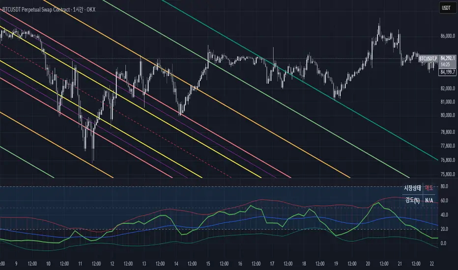
Triple SRSI-MFI Ⅲ - Multi TimeframeTriple SRSI-MFI Ⅲ - Multi Timeframe Indicator
Description
The Triple SRSI-MFI Ⅲ - Multi Timeframe indicator is a powerful tool designed to combine Stochastic RSI (SRSI) and Money Flow Index (MFI) across multiple timeframes (higher, current, and lower). It provides a comprehensive view of market momentum and potential overbought/oversold conditions by calculating a weighted hybrid of SRSI-MFI values from three different timeframes. The indicator also integrates Bollinger Bands to help identify trend direction and volatility.
This indicator is ideal for traders who want to analyze market conditions across multiple timeframes without switching charts. It automatically adjusts settings based on the current timeframe and includes a dynamic weighting system optimized for Bitcoin volatility. Additionally, a real-time information panel displays the market state (buy/sell) and signal strength.
Key Features
Multi-Timeframe Analysis: Combines SRSI-MFI from higher, current, and lower timeframes for a holistic view.
Dynamic Weighting: Automatically adjusts weights for each timeframe based on Bitcoin volatility, with an option for manual customization.
Bollinger Bands Integration: Visualizes trend direction and volatility using Bollinger Bands, with customizable source selection.
Real-Time Info Panel: Displays market state (buy/sell) and signal strength (%) in the top-right corner of the chart.
Customizable Settings: Allows users to tweak MFI source, Bollinger Bands parameters, and visibility of individual components.
How to Use
Add to Chart: Add the "Triple SRSI-MFI Ⅲ - Multi Timeframe" indicator to your chart.
Interpret Signals:
Market State (Buy/Sell): Shown in the info panel. "Buy" when the average SRSI-MFI is above the Bollinger Bands basis, "Sell" when below.
Strength (%): The relative position of the average SRSI-MFI within the Bollinger Bands, scaled from 0% to 100%.
Overbought/Oversold Levels: The indicator plots horizontal lines at 80 (overbought) and 20 (oversold). Use these as potential reversal zones.
Combine with Price Action: Use the indicator in conjunction with price action or other tools for better decision-making.
Adjust Settings: Customize the settings (e.g., Bollinger Bands length, weights, visibility) to match your trading style.
Settings
MFI Source: Select the source for MFI calculation (default: "hlc3"). Options include "close", "open", "high", "low", "hl2", "hlc3", "ohlc4".
Bollinger Bands:
Length: Period for Bollinger Bands calculation (default: 20).
Multiplier: Standard deviation multiplier for the bands (default: 2.0).
Source: Choose which SRSI-MFI value to use for Bollinger Bands ("averageHybrid", "hybrid_higher", "hybrid_current", "hybrid_lower"; default: "hybrid_higher").
Weights:
Auto Weight Enabled: Enable/disable automatic weights based on Bitcoin volatility (default: true).
Higher/Current/Lower Weights: Manually set weights for each timeframe if auto-weight is disabled (defaults: 1.5, 1.0, 0.5).
Indicator On/Off:
Toggle visibility for Higher SRSI-MFI, Current SRSI-MFI, Lower SRSI-MFI, Average SRSI-MFI, and Bollinger Bands.
How It Works
SRSI-MFI Calculation:
Stochastic RSI (SRSI) and Money Flow Index (MFI) are calculated for three timeframes: higher, current, and lower.
The hybrid value (SRSI * (MFI / 100)) is computed for each timeframe.
Weighted Average:
The hybrid values are combined into a weighted average (averageHybrid) using dynamic or manual weights.
Bollinger Bands:
Bollinger Bands are applied to the selected source (e.g., hybrid_higher) to identify trend direction and volatility.
Relative Position:
The position of averageHybrid within the Bollinger Bands is scaled to a percentage (0% to 100%) for strength assessment.
Visualization:
Plots individual SRSI-MFI lines, Bollinger Bands, and overbought/oversold levels.
A real-time info panel provides market state and signal strength.
Notes
This indicator is best used as part of a broader trading strategy. It is not a standalone signal generator and should be combined with other forms of analysis.
The automatic weights are optimized for Bitcoin (BTC) volatility. For other assets, you may need to adjust the weights manually.
The indicator may require sufficient historical data to calculate higher and lower timeframe values accurately.
Buscar en scripts para "通达信+选股公式+换手率+0.5+源码"
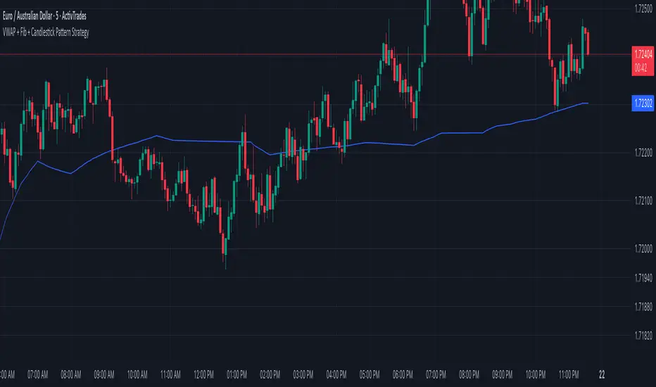
VWAP + Fib + Candlestick Pattern Strategy### **VWAP + Fibonacci + Candlestick Pattern Strategy (v6)**
This indicator is designed to identify high-quality trading setups using a combination of **Anchored VWAP, Fibonacci Retracement Levels, and Candlestick Patterns**. It helps traders find optimal entry points where multiple confluences align, enhancing trade accuracy.
### **Key Features:**
✅ **Anchored VWAP** – Starts from the last pivot low (bullish) or pivot high (bearish) to determine trend strength.
✅ **Fibonacci Levels** – Uses key retracement levels (0.382, 0.5, 0.618, 0.786) for added confluence.
✅ **Candlestick Patterns** – Detects Pin Bars, Engulfing Candles, and Hammer Candles for potential reversals.
✅ **High-Quality Setups** – Highlights strong signals where price aligns with VWAP & Fib zones.
✅ **Alerts** – Get notified when a bullish or bearish setup is detected.
✅ **Risk Management** – Includes Take Profit (TP1, TP2, Final TP) & Stop Loss based on ATR.
✅ **Position Sizing** – Calculates position size based on a fixed dollar risk per trade.
### **How to Use:**
1. Apply the indicator to your chart.
2. Look for signals near Fibonacci retracement levels and VWAP.
3. Use alerts for real-time trade notifications.
4. Manage risk with built-in TP/SL and position sizing.
Perfect for traders who use **Price Action & Smart Money Concepts** to refine their entries! 🚀
Double Bollinger Bands MTF and Price projectionI did this script because I wanted to project prices over future bars quickly because I am a options trader.
Options:
Time frame: Default is Chart
Some times I prefer using 15 m with period 200 on a daily chart in a fast moving market. But you can chose what suites you
BB inner deviation 1 is default
When BB inner deviation=1 the outer will be 2X if its 0.5 outer will be 1
Moving Average type : Default EMA
Project next bar in label Default is off
This will calculate a linear projection of price of each band for the number of bars requested and print them in the label. It does not plot the future values
Using: in a trending market the prices will be generally be between band1 and band 2
and other times between -band1 and +band1. The projection can assist in optimal option strategy. Also in a fast moving market I would use 10 period ema for accurate price projections and others 20

Elastic Volume-Weighted Student-T TensionOverview
The Elastic Volume-Weighted Student-T Tension Bands indicator dynamically adapts to market conditions using an advanced statistical model based on the Student-T distribution. Unlike traditional Bollinger Bands or Keltner Channels, this indicator leverages elastic volume-weighted averaging to compute real-time dispersion and location parameters, making it highly responsive to volatility changes while maintaining robustness against price fluctuations.
This methodology is inspired by incremental calculation techniques for weighted mean and variance, as outlined in the paper by Tony Finch:
📄 "Incremental Calculation of Weighted Mean and Variance" .
Key Features
✅ Adaptive Volatility Estimation – Uses an exponentially weighted Student-T model to dynamically adjust band width.
✅ Volume-Weighted Mean & Dispersion – Incorporates real-time volume weighting, ensuring a more accurate representation of market sentiment.
✅ High-Timeframe Volume Normalization – Provides an option to smooth volume impact by referencing a higher timeframe’s cumulative volume, reducing noise from high-variability bars.
✅ Customizable Tension Parameters – Configurable standard deviation multipliers (σ) allow for fine-tuned volatility sensitivity.
✅ %B-Like Oscillator for Relative Price Positioning – The main indicator is in form of a dedicated oscillator pane that normalizes price position within the sigma ranges, helping identify overbought/oversold conditions and potential momentum shifts.
✅ Robust Statistical Foundation – Utilizes kurtosis-based degree-of-freedom estimation, enhancing responsiveness across different market conditions.
How It Works
Volume-Weighted Elastic Mean (eμ) – Computes a dynamic mean price using an elastic weighted moving average approach, influenced by trade volume, if not volume detected in series, study takes true range as replacement.
Dispersion (eσ) via Student-T Distribution – Instead of assuming a fixed normal distribution, the bands adapt to heavy-tailed distributions using kurtosis-driven degrees of freedom.
Incremental Calculation of Variance – The indicator applies Tony Finch’s incremental method for computing weighted variance instead of arithmetic sum's of fixed bar window or arrays, improving efficiency and numerical stability.
Tension Calculation – There are 2 dispersion custom "zones" that are computed based on the weighted mean and dynamically adjusted standard student-t deviation.
%B-Like Oscillator Calculation – The oscillator normalizes the price within the band structure, with values between 0 and 1:
* 0.00 → Price is at the lower band (-2σ).
* 0.50 → Price is at the volume-weighted mean (eμ).
* 1.00 → Price is at the upper band (+2σ).
* Readings above 1.00 or below 0.00 suggest extreme movements or possible breakouts.
Recommended Usage
For scalping in lower timeframes, it is recommended to use the fixed α Decay Factor, it is in raw format for better control, but you can easily make a like of transformation to N-bar size window like in EMA-1 bar dividing 2 / decayFactor or like an RMA dividing 1 / decayFactor.
The HTF selector catch quite well Higher Time Frame analysis, for example using a Daily chart and using as HTF the 200-day timeframe, weekly or monthly.
Suitable for trend confirmation, breakout detection, and mean reversion plays.
The %B-like oscillator helps gauge momentum strength and detect divergences in price action if user prefer a clean chart without bands, this thanks to pineScript v6 force overlay feature.
Ideal for markets with volume-driven momentum shifts (e.g., futures, forex, crypto).
Customization Parameters
Fixed α Decay Factor – Controls the rate of volume weighting influence for an approximation EWMA approach instead of using sum of series or arrays, making the code lightweight & computing fast O(1).
HTF Volume Smoothing – Instead of a fixed denominator for computing α , a volume sum of the last 2 higher timeframe closed candles are used as denominator for our α weight factor. This is useful to review mayor trends like in daily, weekly, monthly.
Tension Multipliers (±σ) – Adjusts sensitivity to dispersion sigma parameter (volatility).
Oscillator Zone Fills – Visual cues for price positioning within the cloud range.
Posible Interpretations
As market within indicators relay on each individual edge, this are just some key ideas to glimpse how the indicator could be interpreted by the user:
📌 Price inside bands – Market is considered somehow "stable"; price is like resting from tension or "charging batteries" for volume spike moves.
📌 Price breaking outer bands – Potential breakout or extreme movement; watch for reversals or continuation from strong moves. Market is already in tension or generating it.
📌 Narrowing Bands – Decreasing volatility; expect contraction before expansion.
📌 Widening Bands – Increased volatility; prepare for high probability pull-back moves, specially to the center location of the bands (the mean) or the other side of them.
📌 Oscillator is just the interpretation of the price normalized across the Student-T distribution fitting "curve" using the location parameter, our Elastic Volume weighted mean (eμ) fixed at 0.5 value.
Final Thoughts
The Elastic Volume-Weighted Student-T Tension indicator provides a powerful, volume-sensitive alternative to traditional volatility bands. By integrating real-time volume analysis with an adaptive statistical model, incremental variance computation, in a relative price oscillator that can be overlayed in the chart as bands, it offers traders an edge in identifying momentum shifts, trend strength, and breakout potential. Think of the distribution as a relative "tension" rubber band in which price never leave so far alone.
DISCLAIMER:
The Following indicator/code IS NOT intended to be a formal investment advice or recommendation by the author, nor should be construed as such. Users will be fully responsible by their use regarding their own trading vehicles/assets.
The following indicator was made for NON LUCRATIVE ACTIVITIES and must remain as is, following TradingView's regulations. Use of indicator and their code are published for work and knowledge sharing. All access granted over it, their use, copy or re-use should mention authorship(s) and origin(s).
WARNING NOTICE!
THE INCLUDED FUNCTION MUST BE CONSIDERED FOR TESTING. The models included in the indicator have been taken from open sources on the web and some of them has been modified by the author, problems could occur at diverse data sceneries, compiler version, or any other externality.

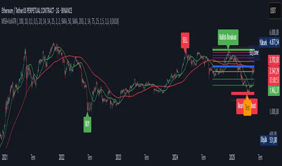
Market Structure Break with Volume & ATR#### Indicator Overview:
The *Market Structure Break with Volume & ATR (MSB+VolATR)* indicator is designed to identify significant market structure breakouts and breakdowns using a combination of price action, volume analysis, and volatility (ATR). It is particularly useful for traders who rely on higher timeframes for swing trading or positional trading. The indicator highlights bullish and bearish breakouts, retests, fakeouts, and potential buy/sell signals based on RSI overbought/oversold conditions.
---
### Key Features:
1. *Market Structure Analysis*:
- Identifies swing highs and lows on a user-defined higher timeframe.
- Detects breakouts and breakdowns when price exceeds these levels with volume and ATR validation.
2. *Volume Validation*:
- Ensures breakouts are accompanied by above-average volume, reducing the likelihood of false signals.
3. *ATR Filter*:
- Filters out insignificant breakouts by requiring the breakout size to exceed a multiple of the ATR.
4. *RSI Integration*:
- Adds a momentum filter by considering overbought/oversold conditions using RSI.
5. *Visual Enhancements*:
- Draws colored boxes to highlight breakout zones.
- Labels breakouts, retests, and fakeouts for easy interpretation.
- Displays stop levels for potential trades.
6. *Alerts*:
- Provides alert conditions for buy and sell signals, enabling real-time notifications.
---
### Input Settings and Their Effects:
1. **Timeframe (tf):
- Determines the higher timeframe for market structure analysis.
- *Effect*: A higher timeframe (e.g., 1D) reduces noise and provides more reliable swing points, while a lower timeframe (e.g., 4H) may generate more frequent but less reliable signals.
2. **Lookback Period (length):
- Defines the number of historical bars used to identify significant highs and lows.
- *Effect*: A longer lookback period (e.g., 50) captures broader market structure, while a shorter period (e.g., 20) reacts faster to recent price action.
3. **ATR Length (atr_length):
- Sets the period for ATR calculation.
- *Effect*: A shorter ATR length (e.g., 14) reacts faster to recent volatility, while a longer length (e.g., 21) smooths out volatility spikes.
4. **ATR Multiplier (atr_multiplier):
- Filters insignificant breakouts by requiring the breakout size to exceed ATR × multiplier.
- *Effect*: A higher multiplier (e.g., 0.2) reduces false signals but may miss smaller breakouts.
5. **Volume Multiplier (volume_multiplier):
- Sets the volume threshold for breakout validation.
- *Effect*: A higher multiplier (e.g., 1.0) ensures stronger volume confirmation but may reduce the number of signals.
6. **RSI Length (rsi_length):
- Defines the period for RSI calculation.
- *Effect*: A shorter RSI length (e.g., 10) makes the indicator more sensitive to recent price changes, while a longer length (e.g., 20) smooths out RSI fluctuations.
7. *RSI Overbought/Oversold Levels*:
- Sets the thresholds for overbought (default: 70) and oversold (default: 30) conditions.
- *Effect*: Adjusting these levels can make the indicator more or less conservative in generating signals.
8. **Stop Loss Multiplier (SL_Multiplier):
- Determines the distance of the stop-loss level from the entry price based on ATR.
- *Effect*: A higher multiplier (e.g., 2.0) provides wider stops, reducing the risk of being stopped out prematurely but increasing potential losses.
---
### How It Works:
1. *Breakout Detection*:
- A bullish breakout occurs when the close exceeds the highest high of the lookback period, with volume above the threshold and breakout size exceeding ATR × multiplier.
- A bearish breakout occurs when the close falls below the lowest low of the lookback period, with similar volume and ATR validation.
2. *Retest Logic*:
- After a breakout, if price retests the breakout zone without closing beyond it, a retest label is displayed.
3. *Fakeout Detection*:
- If price briefly breaks out but reverses back into the range, a fakeout label is displayed.
4. *Buy/Sell Signals*:
- A sell signal is generated when price reverses below a bullish breakout zone and RSI is overbought.
- A buy signal is generated when price reverses above a bearish breakout zone and RSI is oversold.
5. *Stop Levels*:
- Stop-loss levels are plotted based on ATR × SL_Multiplier, providing a visual guide for risk management.
---
### Who Can Use It and How:
1. *Swing Traders*:
- Use the indicator on daily or 4-hour timeframes to identify high-probability breakout trades.
- Combine with other technical analysis tools (e.g., trendlines, Fibonacci levels) for confirmation.
2. *Positional Traders*:
- Apply the indicator on weekly or daily charts to capture long-term trends.
- Use the stop-loss levels to manage risk over extended periods.
3. *Algorithmic Traders*:
- Integrate the buy/sell signals into automated trading systems.
- Use the alert conditions to trigger trades programmatically.
4. *Risk-Averse Traders*:
- Adjust the ATR and volume multipliers to filter out low-probability trades.
- Use wider stop-loss levels to avoid premature exits.
---
### Where to Use It:
- *Forex*: Identify breakouts in major currency pairs.
- *Stocks*: Spot trend reversals in high-volume stocks.
- *Commodities*: Trade breakouts in gold, oil, or other commodities.
- *Crypto*: Apply to Bitcoin, Ethereum, or other cryptocurrencies for volatile breakout opportunities.
---
### Example Use Case:
- *Timeframe*: 1D
- *Lookback Period*: 50
- *ATR Length*: 14
- *ATR Multiplier*: 0.1
- *Volume Multiplier*: 0.5
- *RSI Length*: 14
- *RSI Overbought/Oversold*: 70/30
- *SL Multiplier*: 1.5
In this setup, the indicator will:
1. Identify significant swing highs and lows on the daily chart.
2. Validate breakouts with volume and ATR filters.
3. Generate buy/sell signals when price reverses and RSI confirms overbought/oversold conditions.
4. Plot stop-loss levels for risk management.
---
### Conclusion:
The *MSB+VolATR* indicator is a versatile tool for traders seeking to capitalize on market structure breakouts with added confirmation from volume and volatility. By customizing the input settings, traders can adapt the indicator to their preferred trading style and risk tolerance. Whether you're a swing trader, positional trader, or algorithmic trader, this indicator provides actionable insights to enhance your trading strategy.
Fibonacci - DolphinTradeBot
OVERVIEW
The 'Fibonacci - DolphinTradeBot' indicator is a Pine Script-based tool for TradingView that dynamically identifies key Fibonacci retracement levels using ZigZag price movements. It aims to replicate the Fibonacci Retracement tool available in TradingView’s drawing tools. The indicator calculates Fibonacci levels based on directional price changes, marking critical retracement zones such as 0, 0.236, 0.382, 0.5, 0.618, 0.786, and 1.0 on the chart. These levels are visualized with lines and labels, providing traders with precise areas of potential price reversals or trend continuation.
HOW IT WORKS ?
The indicator follows a zigzag formation. After a large swing movement, when new swings are formed without breaking the upper and lower levels, it places Fibonacci levels at the beginning and end points of the major swing movement."
▪️(Bullish) Structure :High → HigherLow → LowerHigh
▪️(Bearish) Structure :Low → LowerHigh → HigherLow
▪️When Fibonacci retracement levels are determined, a "📌" mark appears on the chart.
▪️If the price closes outside of these levels, a "❌" mark will appear.
USAGE
This indicator is designed to plot Fibonacci levels within an accumulation zone following significant price movements, helping you identify potential support and resistance. You can adjust the pivot periods to customize the zigzag settings to your preference. While classic Fibonacci levels are used by default, you also have the option to input custom levels and assign your preferred colors.
Set the Fibonacci direction option to "upward" to detect only bullish structures, "downward" to detect only bearish structures, and "both" to see both at the same time.
"To view past levels, simply enable the ' Show Previous Levels ' option, and to display the zigzag lines, activate the ' Show Zigzag ' setting."
ALERTS
The indicator, by default, triggers an alarm when both a level is formed and when a level is broken. However, if you'd like, you can select the desired level from the " Select Level " section in the indicator settings and set the alarm based on one of the conditions below.
▪️ cross-up → If the price breaks the Fibonacci level to the upside.
▪️ cross-down → If the price breaks the Fibonacci level to the downside.
▪️ cross-any → If the price breaks the Fibonacci level in any direction.

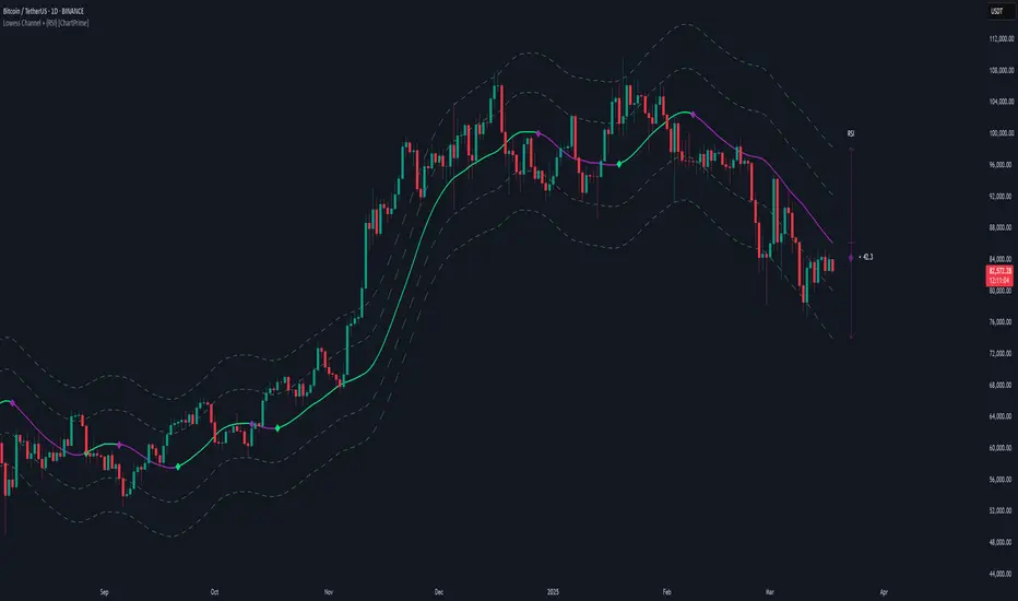
Lowess Channel + (RSI) [ChartPrime]The Lowess Channel + (RSI) indicator applies the LOWESS (Locally Weighted Scatterplot Smoothing) algorithm to filter price fluctuations and construct a dynamic channel. LOWESS is a non-parametric regression method that smooths noisy data by fitting weighted linear regressions at localized segments. This technique is widely used in statistical analysis to reveal trends while preserving data structure.
In this indicator, the LOWESS algorithm is used to create a central trend line and deviation-based bands. The midline changes color based on trend direction, and diamonds are plotted when a trend shift occurs. Additionally, an RSI gauge is positioned at the end of the channel to display the current RSI level in relation to the price bands.
lowess_smooth(src, length, bandwidth) =>
sum_weights = 0.0
sum_weighted_y = 0.0
sum_weighted_xy = 0.0
sum_weighted_x2 = 0.0
sum_weighted_x = 0.0
for i = 0 to length - 1
x = float(i)
weight = math.exp(-0.5 * (x / bandwidth) * (x / bandwidth))
y = nz(src , 0)
sum_weights := sum_weights + weight
sum_weighted_x := sum_weighted_x + weight * x
sum_weighted_y := sum_weighted_y + weight * y
sum_weighted_xy := sum_weighted_xy + weight * x * y
sum_weighted_x2 := sum_weighted_x2 + weight * x * x
mean_x = sum_weighted_x / sum_weights
mean_y = sum_weighted_y / sum_weights
beta = (sum_weighted_xy - mean_x * mean_y * sum_weights) / (sum_weighted_x2 - mean_x * mean_x * sum_weights)
alpha = mean_y - beta * mean_x
alpha + beta * float(length / 2) // Centered smoothing
⯁ KEY FEATURES
LOWESS Price Filtering – Smooths price fluctuations to reveal the underlying trend with minimal lag.
Dynamic Trend Coloring – The midline changes color based on trend direction (e.g., bullish or bearish).
Trend Shift Diamonds – Marks points where the midline color changes, indicating a possible trend shift.
Deviation-Based Bands – Expands above and below the midline using ATR-based multipliers for volatility tracking.
RSI Gauge Display – A vertical gauge at the right side of the chart shows the current RSI level relative to the price channel.
Fully Customizable – Users can adjust LOWESS length, band width, colors, and enable or disable the RSI gauge and adjust RSIlength.
⯁ HOW TO USE
Use the LOWESS midline as a trend filter —bullish when green, bearish when purple.
Watch for trend shift diamonds as potential entry or exit signals.
Utilize the price bands to gauge overbought and oversold zones based on volatility.
Monitor the RSI gauge to confirm trend strength—high RSI near upper bands suggests overbought conditions, while low RSI near lower bands indicates oversold conditions.
⯁ CONCLUSION
The Lowess Channel + (RSI) indicator offers a powerful way to analyze market trends by applying a statistically robust smoothing algorithm. Unlike traditional moving averages, LOWESS filtering provides a flexible, responsive trendline that adapts to price movements. The integrated RSI gauge enhances decision-making by displaying momentum conditions alongside trend dynamics. Whether used for trend-following or mean reversion strategies, this indicator provides traders with a well-rounded perspective on market behavior.
Liquidity Zones [ActiveQuants]The Liquidity Zones indicator detects price areas where high trading volume coincides with below-average volatility , critical zones where large players often accumulate or distribute positions. Ideal for spotting potential reversal points and strategic liquidity pools.
Core Detection Formula
Liquidity Zone = (Volume > SMA(Volume, Length) × Multiplier) AND (Short-Term Volatility < 0.5 × Average Volatility)
Volume Surge Detection
Compares current volume to its SMA (user-defined length).
Multiplies threshold with " Volume Threshold Multiplier " parameter.
Volatility Contraction Filter
Calculates 5-bar volatility (standard deviation of closes).
Compares to average volatility over " Price Std. Dev. Length " period.
Requires short-term volatility < 50% of average.
█ KEY FEATURES
Merging Consecutive Zones
If the " Merge Consecutive Zones " option is enabled, the indicator will:
Calculate the number of consecutive bars that meet the liquidity zone criteria.
Sum the volume of these consecutive bars.
Display only the most recent label for the merged zone (previous labels in the sequence are removed).
Displays volume in either
Raw units (" Units ").
Dollar-equivalent (" Currency Value ") using closing price.
Alerts
An alert condition is built into the script. Traders can selectively enable alerts via TradingView’s alert system. Whenever a liquidity zone is detected, an alert is triggered with the message: " High-volume and low-volatility zone detected! ".
█ USER INPUTS
- Liquidity Zones Color
Sets the background color for liquidity zones.
Default: Orange (with 70 transparency).
- Volume SMA Length
Determines the number of bars over which the volume simple moving average is calculated.
Default: 20 bars.
- Volume Threshold Multiplier
Multiplies the volume SMA to establish a threshold. A bar’s volume must exceed this product to be considered high volume.
Default: 2.0.
- Price Std. Dev. Length
The period used to calculate the standard deviation of the closing prices. This is the basis for measuring average volatility.
Default: 14 bars.
- Zone Volume
A toggle to display a label with the volume value on liquidity zones.
Allows you to choose how the volume is displayed: Units (shows raw volume) or Currency Value (multiplies volume by the current closing price).
Allows you to choose the font size of the volume label.
- Merge Consecutive Zones
When enabled, volumes from consecutive liquidity zones are summed into a single total, and only the most recent label is displayed (previous labels in the sequence are removed).
Default: Enabled.
- Show Last
Specifies the number of bars back that the indicator will evaluate and plot liquidity zones.
Default: 500 bars.
- Timeframe
Analysis period.
Default: Chart.
█ CONCLUSION
The Liquidity Zones indicator is a powerful tool for traders seeking to identify key areas on the chart where liquidity is concentrated, characterized by high volume and low volatility . With customizable settings for volume analysis and volatility measurement , this indicator can be integrated into a wide range of trading strategies. It not only highlights these zones visually but also provides volume data labels and alerts for timely decision-making.
█ IMPORTANT NOTES
⚠ Volume and Volatility Settings: Adjust the Volume SMA Length , Volume Threshold Multiplier , and Price Std. Dev. Length to suit the typical trading volume and volatility of the asset you are analyzing.
⚠ Confirmed Bars Only: Signals are generated only on confirmed bars. This minimizes false signals due to intra-bar noise and also prevents indicator repainting .
⚠ Risk Management: Liquidity zones may signal areas of potential accumulation or distribution, but they should be used in conjunction with other technical analysis tools (e.g., support/resistance levels, trendlines, or momentum indicators). Trading involves risk, and it is recommended to combine this indicator with proper risk management techniques.
█ RISK DISCLAIMER
Trading involves substantial risk of loss. Liquidity zones indicate potential interest areas but don't guarantee price reactions. Always confirm with additional analysis and proper risk management. Past performance is not indicative of future results.
📈 Happy trading! 🚀

Opening RangeShows the opening range for morning and afternoon session. 9:30-10:00 and 1:30-2:00 EST.
It also has the option to add 0.5 and 1 standard deviations in both directions or range extensions.
Note: If you are having weird scaling issues when using this script, especially with the extensions, go to the settings in the bottom right of the chart. It is where the time and price axis meet which is bottom right by default. And then make sure "Scale price chart only" is enabled.

Price / 200 SMA Ratio (Pr)Price / 200 SMA Ratio (Pr) Indicator
The Price / 200 SMA Ratio (Pr) indicator is designed to help traders analyze the relationship between the current price and the 200-period Simple Moving Average (SMA). By calculating the ratio of the close price to the 200 SMA, the indicator provides a visual representation of how the price compares to the long-term trend, giving traders a clear view of potential overbought or oversold conditions.
How It Works:
Ratio Calculation:
The core of this indicator lies in the ratio between the current close price and the 200-period Simple Moving Average (SMA). The formula is straightforward:
Ratio = Close Price / 200 SMA
This ratio indicates whether the current price is above or below the long-term trend (the 200 SMA). A ratio greater than 1 means the price is above the 200 SMA, while a ratio below 1 suggests the price is below the 200 SMA.
Color-Coded Ratio Representation:
The ratio is displayed as a line on the chart with a color that changes dynamically based on the value of the ratio. The color-coding system helps quickly identify key levels:
Black: When the ratio is greater than 5, the price is significantly above the 200 SMA, indicating a highly overbought condition.
Red: When the ratio is greater than 3.5, it signals that the price is significantly above the long-term average but not in extreme territory.
Blue: When the ratio is less than 1, the price is below the 200 SMA, indicating that the market may be in an oversold condition.
Purple: When the ratio is below 0.7, it suggests an extremely oversold market, well below the long-term average.
Green: For values in between, the ratio is considered to be in a more neutral range, showing a balanced market position.
Horizontal Reference Lines:
To make the interpretation of the ratio easier, the indicator includes several reference lines plotted at key ratio levels. These lines help traders visualize specific price zones, giving them clear boundaries for potential trading decisions:
5 Zone (Black line): Marks an extremely high price level, indicating a highly overbought condition.
3.5 Zone (Red line): Represents the upper price zone, where prices are significantly higher than the 200 SMA.
2 Zone (Purple line): This line marks the mid-range of the ratio, providing a visual representation of the transition between overbought and oversold conditions.
1 Zone (Orange line): The 1.0 line is where the price equals the 200 SMA, indicating a balanced market. Prices above 1.0 are considered above average, and prices below 1.0 are below average.
0.7 Zone (Blue line): Represents a very low price level, suggesting an extremely oversold market.
Extra Low Zone (Green line): This line marks an even lower price level, indicating severe oversold conditions.
Background Coloring:
In addition to the ratio line and reference lines, the background color of the chart changes dynamically to provide additional context to the trader:
Red Background: When the ratio is greater than 3.5, the background becomes red, signaling an overbought market condition.
Blue Background: When the ratio is less than 1, the background turns blue, indicating a potential oversold market.
Black Background: If the ratio exceeds 5, the background will be black, signifying an extreme overbought condition.
Green Background: If the ratio drops below 0.7, the background turns green, highlighting an extremely oversold market.
Candle Coloring:
The indicator also changes the color of the individual price bars (candles) based on the ratio value:
Black Candles: When the ratio is greater than 5 or less than 0.7, the price bars are black to emphasize extreme conditions in the market.
White Candles: For all other values, the candles are white, representing a neutral market condition.
What This Indicator Tells You:
Overbought Conditions: When the ratio is significantly above 1 (especially greater than 3.5 or 5), it indicates that the price is far above the 200 SMA, suggesting that the market may be overbought and could experience a correction.
Oversold Conditions: When the ratio is significantly below 1 (especially below 0.7 or 0.5), it suggests that the price is far below the 200 SMA, indicating that the market may be oversold and could be due for a bounce.
Trend and Momentum: The ratio provides insight into the overall trend. If the ratio is consistently above 1, it means the price is generally in an uptrend, and if it’s below 1, it indicates a downtrend.
Why Use This Indicator?
The Price / 200 SMA Ratio indicator is a valuable tool for traders who want to gain insights into the strength or weakness of the price relative to the long-term trend (200 SMA). The color-coding system provides an easy-to-read visual cue, and the reference lines allow traders to identify key price levels where potential reversal or continuation could occur. It helps to spot areas of overbought or oversold conditions, making it ideal for traders looking to enter or exit positions based on extreme price movements.
By combining this indicator with other technical analysis tools, traders can enhance their strategy and make more informed decisions in the market.

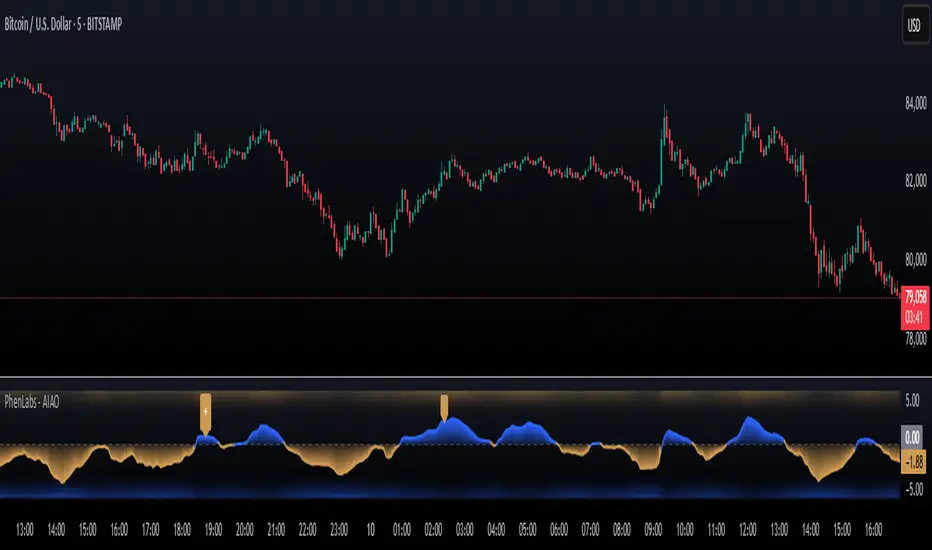
AI Adaptive Oscillator [PhenLabs]📊 Algorithmic Adaptive Oscillator
Version: PineScript™ v6
📌 Description
The AI Adaptive Oscillator is a sophisticated technical indicator that employs ensemble learning and adaptive weighting techniques to analyze market conditions. This innovative oscillator combines multiple traditional technical indicators through an AI-driven approach that continuously evaluates and adjusts component weights based on historical performance. By integrating statistical modeling with machine learning principles, the indicator adapts to changing market dynamics, providing traders with a responsive and reliable tool for market analysis.
🚀 Points of Innovation:
Ensemble learning framework with adaptive component weighting
Performance-based scoring system using directional accuracy
Dynamic volatility-adjusted smoothing mechanism
Intelligent signal filtering with cooldown and magnitude requirements
Signal confidence levels based on multi-factor analysis
🔧 Core Components
Ensemble Framework : Combines up to five technical indicators with performance-weighted integration
Adaptive Weighting : Continuous performance evaluation with automated weight adjustment
Volatility-Based Smoothing : Adapts sensitivity based on current market volatility
Pattern Recognition : Identifies potential reversal patterns with signal qualification criteria
Dynamic Visualization : Professional color schemes with gradient intensity representation
Signal Confidence : Three-tiered confidence assessment for trading signals
🔥 Key Features
The indicator provides comprehensive market analysis through:
Multi-Component Ensemble : Integrates RSI, CCI, Stochastic, MACD, and Volume-weighted momentum
Performance Scoring : Evaluates each component based on directional prediction accuracy
Adaptive Smoothing : Automatically adjusts based on market volatility
Pattern Detection : Identifies potential reversal patterns in overbought/oversold conditions
Signal Filtering : Prevents excessive signals through cooldown periods and minimum change requirements
Confidence Assessment : Displays signal strength through intuitive confidence indicators (average, above average, excellent)
🎨 Visualization
Gradient-Filled Oscillator : Color intensity reflects strength of market movement
Clear Signal Markers : Distinct bullish and bearish pattern signals with confidence indicators
Range Visualization : Clean representation of oscillator values from -6 to 6
Zero Line : Clear demarcation between bullish and bearish territory
Customizable Colors : Color schemes that can be adjusted to match your chart style
Confidence Symbols : Intuitive display of signal confidence (no symbol, +, or ++) alongside direction markers
📖 Usage Guidelines
⚙️ Settings Guide
Color Settings
Bullish Color
Default: #2b62fa (Blue)
This setting controls the color representation for bullish movements in the oscillator. The color appears when the oscillator value is positive (above zero), with intensity indicating the strength of the bullish momentum. A brighter shade indicates stronger bullish pressure.
Bearish Color
Default: #ce9851 (Amber)
This setting determines the color representation for bearish movements in the oscillator. The color appears when the oscillator value is negative (below zero), with intensity reflecting the strength of the bearish momentum. A more saturated shade indicates stronger bearish pressure.
Signal Settings
Signal Cooldown (bars)
Default: 10
Range: 1-50
This parameter sets the minimum number of bars that must pass before a new signal of the same type can be generated. Higher values reduce signal frequency and help prevent overtrading during choppy market conditions. Lower values increase signal sensitivity but may generate more false positives.
Min Change For New Signal
Default: 1.5
Range: 0.5-3.0
This setting defines the minimum required change in oscillator value between consecutive signals of the same type. It ensures that new signals represent meaningful changes in market conditions rather than minor fluctuations. Higher values produce fewer but potentially higher-quality signals, while lower values increase signal frequency.
AI Core Settings
Base Length
Default: 14
Minimum: 2
This fundamental setting determines the primary calculation period for all technical components in the ensemble (RSI, CCI, Stochastic, etc.). It represents the lookback window for each component’s base calculation. Shorter periods create a more responsive but potentially noisier oscillator, while longer periods produce smoother signals with potential lag.
Adaptive Speed
Default: 0.1
Range: 0.01-0.3
Controls how quickly the oscillator adapts to new market conditions through its volatility-adjusted smoothing mechanism. Higher values make the oscillator more responsive to recent price action but potentially more erratic. Lower values create smoother transitions but may lag during rapid market changes. This parameter directly influences the indicator’s adaptiveness to market volatility.
Learning Lookback Period
Default: 150
Minimum: 10
Determines the historical data range used to evaluate each ensemble component’s performance and calculate adaptive weights. This setting controls how far back the AI “learns” from past performance to optimize current signals. Longer periods provide more stable weight distribution but may be slower to adapt to regime changes. Shorter periods adapt more quickly but may overreact to recent anomalies.
Ensemble Size
Default: 5
Range: 2-5
Specifies how many technical components to include in the ensemble calculation.
Understanding The Interaction Between Settings
Base Length and Learning Lookback : The base length determines the reactivity of individual components, while the lookback period determines how their weights are adjusted. These should be balanced according to your timeframe - shorter timeframes benefit from shorter base lengths, while the lookback should generally be 10-15 times the base length for optimal learning.
Adaptive Speed and Signal Cooldown : These settings control sensitivity from different angles. Increasing adaptive speed makes the oscillator more responsive, while reducing signal cooldown increases signal frequency. For conservative trading, keep adaptive speed low and cooldown high; for aggressive trading, do the opposite.
Ensemble Size and Min Change : Larger ensembles provide more stable signals, allowing for a lower minimum change threshold. Smaller ensembles might benefit from a higher threshold to filter out noise.
Understanding Signal Confidence Levels
The indicator provides three distinct confidence levels for both bullish and bearish signals:
Average Confidence (▲ or ▼) : Basic signal that meets the minimum pattern and filtering criteria. These signals indicate potential reversals but with moderate confidence in the prediction. Consider using these as initial alerts that may require additional confirmation.
Above Average Confidence (▲+ or ▼+) : Higher reliability signal with stronger underlying metrics. These signals demonstrate greater consensus among the ensemble components and/or stronger historical performance. They offer increased probability of successful reversals and can be traded with less additional confirmation.
Excellent Confidence (▲++ or ▼++) : Highest quality signals with exceptional underlying metrics. These signals show strong agreement across oscillator components, excellent historical performance, and optimal signal strength. These represent the indicator’s highest conviction trade opportunities and can be prioritized in your trading decisions.
Confidence assessment is calculated through a multi-factor analysis including:
Historical performance of ensemble components
Degree of agreement between different oscillator components
Relative strength of the signal compared to historical thresholds
✅ Best Use Cases:
Identify potential market reversals through oscillator extremes
Filter trade signals based on AI-evaluated component weights
Monitor changing market conditions through oscillator direction and intensity
Confirm trade signals from other indicators with adaptive ensemble validation
Detect early momentum shifts through pattern recognition
Prioritize trading opportunities based on signal confidence levels
Adjust position sizing according to signal confidence (larger for ++ signals, smaller for standard signals)
⚠️ Limitations
Requires sufficient historical data for accurate performance scoring
Ensemble weights may lag during dramatic market condition changes
Higher ensemble sizes require more computational resources
Performance evaluation quality depends on the learning lookback period length
Even high confidence signals should be considered within broader market context
💡 What Makes This Unique
Adaptive Intelligence : Continuously adjusts component weights based on actual performance
Ensemble Methodology : Combines strength of multiple indicators while minimizing individual weaknesses
Volatility-Adjusted Smoothing : Provides appropriate sensitivity across different market conditions
Performance-Based Learning : Utilizes historical accuracy to improve future predictions
Intelligent Signal Filtering : Reduces noise and false signals through sophisticated filtering criteria
Multi-Level Confidence Assessment : Delivers nuanced signal quality information for optimized trading decisions
🔬 How It Works
The indicator processes market data through five main components:
Ensemble Component Calculation :
Normalizes traditional indicators to consistent scale
Includes RSI, CCI, Stochastic, MACD, and volume components
Adapts based on the selected ensemble size
Performance Evaluation :
Analyzes directional accuracy of each component
Calculates continuous performance scores
Determines adaptive component weights
Oscillator Integration :
Combines weighted components into unified oscillator
Applies volatility-based adaptive smoothing
Scales final values to -6 to 6 range
Signal Generation :
Detects potential reversal patterns
Applies cooldown and magnitude filters
Generates clear visual markers for qualified signals
Confidence Assessment :
Evaluates component agreement, historical accuracy, and signal strength
Classifies signals into three confidence tiers (average, above average, excellent)
Displays intuitive confidence indicators (no symbol, +, ++) alongside direction markers
💡 Note:
The AI Adaptive Oscillator performs optimally when used with appropriate timeframe selection and complementary indicators. Its adaptive nature makes it particularly valuable during changing market conditions, where traditional fixed-weight indicators often lose effectiveness. The ensemble approach provides a more robust analysis by leveraging the collective intelligence of multiple technical methodologies. Pay special attention to the signal confidence indicators to optimize your trading decisions - excellent (++) signals often represent the most reliable trade opportunities.
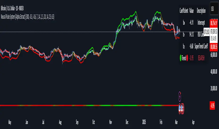
Neural Pulse System [Alpha Extract]Neural Pulse System (NPS)
The Neural Pulse System (NPS) is a custom technical indicator that analyzes price action through a probabilistic lens, offering a dynamic view of bullish and bearish tendencies.
Unlike traditional binary classification models, NPS employs Ordinary Least Squares (OLS) regression with dynamically computed coefficients to produce a smooth probability output ranging from -1 to 1.
Paired with ATR-based bands, this indicator provides an intuitive and volatility-aware approach to trend analysis.
🔶 CALCULATION
The Neural Pulse System utilizes OLS regression to compute probabilities of bullish or bearish price action while incorporating ATR-based bands for volatility context:
Dynamic Coefficients: Coefficients are recalculated in real-time and scaled up to ensure the regression adapts to evolving market conditions.
Ordinary Least Squares (OLS): Uses OLS regression instead of gradient descent for more precise and efficient coefficient estimation.
ATR Bands: Smoothed Average True Range (ATR) bands serve as dynamic boundaries, framing the regression within market volatility.
Probability Output: Instead of a binary result, the output is a continuous probability curve (-1 to 1), helping traders gauge the strength of bullish or bearish momentum.
Formula:
OLS Regression = Line of best fit minimizing squared errors
Probability Signal = Transformed regression output scaled to -1 (bearish) to 1 (bullish)
ATR Bands = Smoothed Average True Range (ATR) to frame price movements within market volatility
🔶 DETAILS
📊 Visual Features:
Probability Curve: Smooth probability signal ranging from -1 (bearish) to 1 (bullish)
ATR Bands: Price action is constrained within volatility bands, preventing extreme deviations
Color-Coded Signals:
Blue to Green: Increasing probability of bullish momentum
Orange to Red: Increasing probability of bearish momentum
Interpretation:
Bullish Bias: Probability output consistently above 0 suggests a bullish trend.
Bearish Bias: Probability output consistently below 0 indicates bearish pressure.
Reversals: Extreme values near -1 or 1, followed by a move toward 0, may signal potential trend reversals.
🔶 EXAMPLES
📌 Trend Identification: Use the probability output to gauge trend direction.
📌Example: On a 1-hour chart, NPS moves from -0.5 to 0.8 as price breaks resistance, signaling a bullish trend.
Reversal Signals: Watch for probability extremes near -1 or 1 followed by a reversal toward 0.
Example: NPS hits 0.9, price touches the upper ATR band, then both retreat—indicating a potential pullback.
📌 Example snapshots:
Volatility Context: ATR bands help assess whether price action aligns with typical market conditions.
Example: During low volatility, the probability signal hovers near 0, and ATR bands tighten, suggesting a potential breakout.
🔶 SETTINGS
Customization Options:
ATR Period – Defines lookback length for ATR calculation (shorter = more responsive, longer = smoother).
ATR Multiplier – Adjusts band width for better volatility capture.
Regression Length – Controls how many bars feed into the coefficient calculation (longer = smoother, shorter = more reactive).
Scaling Factor – Adjusts the strength of regression coefficients.
Output Smoothing – Option to apply a moving average for a cleaner probability curve
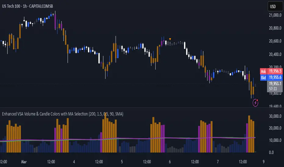
Enhanced VSA Volume & Candle Colors with MA SelectionOverview:
This script aims to enhance the visualization of volume spikes and price action by coloring volume bars and price candles dynamically based on the volume behavior. It allows traders to customize the type of volume moving average (SMA, EMA, or VWMA) used and apply various color schemes to highlight high, low, and extreme volume conditions. Additionally, alerts are generated when extreme or low-volume conditions occur.
---------------------------------------------------------------------------------------------------------------------
Key Features:
Customizable Volume Lookback Period:
The script allows users to define the period for calculating the moving average of volume (default: 200).
Volume Multiplier Settings:
High and low volume thresholds are defined using multipliers. Users can adjust these to customize how volume is categorized (default multipliers: 1.5 for high volume, 0.5 for low volume).
Percentile-Based Extreme Volume Detection:
The script calculates a percentile threshold for extreme volume (default: 90th percentile) based on the volume data, highlighting exceptionally high volume spikes.
Moving Average Selection:
Users can choose between Simple Moving Average (SMA), Exponential Moving Average (EMA), or Volume Weighted Moving Average (VWMA) to track volume trends over the selected lookback period.
Volume-Based Price Bar Coloring:
Price bars can be colored according to the volume conditions (high, low, or extreme). This feature can be toggled on or off.
Dynamic Transparency and Color Customization:
The script allows users to set custom colors for different volume conditions (high, low, neutral, extreme) and adjusts the transparency of volume bars based on the relative size of the volume.
Alerts:
Alerts can be set for when extreme volume spikes or low volume conditions are detected.
---------------------------------------------------------------------------------------------------------------------
Script Components:
Volume Histogram Plot:
Displays the volume bars with dynamic coloring based on the volume condition (high, low, or extreme). The color of the bars adjusts for clarity, with transparency based on volume levels.
Moving Average Plot:
Plots the selected volume moving average (SMA, EMA, or VWMA) to visualize the trend of volume over the chosen lookback period.
Smoothed Average Volume (EMA of Volume):
A smoothed EMA line is plotted to provide a clear representation of volume trends over time.
Price Bar Coloring:
If enabled, price bars are colored according to the current volume condition, providing immediate visual feedback to the trader.
---------------------------------------------------------------------------------------------------------------------
How It Can Be Used:
Volume Analysis for Entry/Exit Points: Traders can use the volume conditions (high, low, and extreme) to identify potential entry or exit points. High-volume bars often signal strong market activity, while low-volume bars may indicate consolidation or indecision.
Volume Confirmation for Trend Reversal: Extreme volume spikes can sometimes precede significant price movements. Traders can monitor these spikes for potential trend reversal signals.
Customizing Alerts: Alerts based on volume conditions help traders stay updated on important volume events without constantly monitoring the chart.
Color-Coded Price Action: The dynamic coloring of price bars makes it easier to identify periods of strong or weak market participation, allowing traders to make informed decisions quickly.
---------------------------------------------------------------------------------------------------------------------
Compliance with TradingView's House Rules:
No Promotion of Financial Products: The script does not promote any specific financial instruments or products, ensuring compliance with TradingView’s content guidelines.
Clear Functionality: The script provides clear, functional analysis tools without making unsupported claims about predicting market movements.
No Automated Trading: The script does not include any automated trading or order execution features, which complies with TradingView’s policy on non-automated scripts.
This breakdown ensures clarity on the script’s purpose, features, and how it might be used by traders. It's written in a way that fits TradingView's content guidelines, keeping the focus on providing valuable analytical tools rather than making promises or promoting any financial product.
Engulfing Sweeps - Milana TradesEngulfing Sweeps
The Engulfing Sweeps Candle is a candlestick pattern that:
1)Takes liquidity from the previous candle’s high or low.
2)Fully engulfs previous candles upon closing.
3)Indicates strong buying or selling pressure.
4)Helps determine the bias of the next candle.
Logic Behind Engulfing Sweeps
If you analyze this candle on a lower timeframe, you’ll often see popular models like PO3 (Power of Three) or AMD (Accumulation – Manipulation – Distribution).
Once the candle closes, the goal is to enter a position on the retracement of the distribution phase.
How to Use Engulfing Sweeps?
Recommended Timeframes:
4H, Daily, Weekly – these levels hold significant liquidity.
Personally, I prefer 4H, as it provides a solid view of mid-term market moves.
Step1 - Identify Engulfing Sweep Candle
Step 2-Switch to a lower timeframe (15m or 5m).And you task identify optimal trade entry
Look for an entry pattern based on:
FVG (Fair Value Gap)
OB (Order Block)
FIB levels (0/0.25/0.5/ 0.75/ 1)
Wait for confirmation and take the trade.
Automating with TradingView Alerts
To avoid missing the pattern, you can set up alerts using a custom script. Once the pattern forms, TradingView will notify you so you can analyze the chart and take action. This approch helps me be more freedom

Auto Fib Retracement [victhoreb]Auto Fib Retracement is an automated Fibonacci retracement tool for TradingView that dynamically identifies key swing points and plots Fibonacci levels to help traders visualize potential support and resistance areas. Using a Zigzag algorithm, the indicator detects recent pivot highs and lows and calculates retracement levels based on these significant price swings. Key features include:
- Dynamic Pivot Detection: Automatically identifies recent swing highs and lows using configurable lookback periods, ensuring the Fibonacci levels adjust as the market evolves.
- Customizable Fibonacci Levels: Users can tailor the Fibonacci retracement levels (0, 0.214, 0.382, 0.5, 0.618, 0.786,) along with individual colors, offering flexibility to match various trading strategies.
- Zigzag Visualization: Optionally displays a Zigzag line that connects the detected pivot points, providing a clear visual representation of the price swing dynamics.
- Adjustable Line Extension: Retracement lines can be extended for a specified number of bars.
- Repainting Option: Includes an option to repaint the Zigzag, ensuring that the most current price action is reflected in the indicator’s output.
- The Auto Fibonacci Retracement itself DOES NOT REPAINT : )
This indicator streamlines the analysis process by automatically drawing Fibonacci retracement levels, allowing traders to quickly identify potential reversal areas and make more informed trading decisions.

Stock Earnings Viewer for Pine ScreenerThe script, titled "Stock Earnings Viewer with Surprise", fetches actual and estimated earnings, calculates absolute and percent surprise values, and presents them for analysis. It is intended to use in Pine Screener, as on chart it is redundant.
How to Apply to Pine Screener
Favorite this script
Open pine screener www.tradingview.com
Select "Stock Earnings Viewer with Surprise" in "Choose indicator"
Click "Scan"
Data
Actual Earnings: The reported earnings per share (EPS) for the stock, sourced via request.earnings().
Estimated Earnings: Analyst-predicted EPS, accessed with field=earnings.estimate.
Absolute Surprise: The difference between actual and estimated earnings (e.g., actual 1.2 - estimated 1.0 = 0.2).
Percent Surprise (%): The absolute surprise as a percentage of estimated earnings (e.g., (0.2 / 1.0) * 100 = 20%). Note: This may return NaN or infinity if estimated earnings are zero, due to division by zero.
Practical Use
This screener script allows users to filter stocks based on earnings metrics. For example, you could screen for stocks where Percent Surprise > 15 to find companies exceeding analyst expectations significantly, or use Absolute Surprise < -0.5 to identify underperformers.

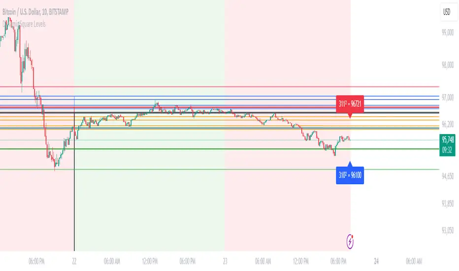
Dynamic Square Levels**Dynamic Square Levels with Strict Range Condition**
This script is designed to help traders visualize dynamic price levels based on the square root of the current price. It calculates key levels above and below the current price, providing a clear view of potential support and resistance zones. The script is highly customizable, allowing you to adjust the number of levels, line styles, and label settings to suit your trading strategy.
---
### **Key Features**:
1. **Dynamic Square Levels**:
- Calculates price levels based on the square root of the current price.
- Plots levels above and below the current price for better market context.
2. **Range Condition**:
- Lines are only drawn when the current price is closer to the base level (`square(base_n)`) than to the next level (`square(base_n + 1)`).
- Ensures levels are only visible when they are most relevant.
3. **Customizable Levels**:
- Choose the number of levels to plot (up to 20 levels).
- Toggle additional levels (e.g., 0.25, 0.5, 0.75) for more granular analysis.
4. **Line and Label Customization**:
- Adjust line width, style (solid, dashed, dotted), and extend direction (left, right, both, or none).
- Customize label text, size, and position for better readability.
5. **Background Highlight**:
- Highlights the background when the current price is closer to the base level, providing a visual cue for key price zones.
---
### **How It Works**:
- The script calculates the square root of the current price and uses it to generate dynamic levels.
- Levels are plotted above and below the current price, with customizable spacing.
- Lines and labels are only drawn when the current price is within a specific range, ensuring clean and relevant visuals.
---
### **Why Use This Script?**:
- **Clear Visuals**: Easily identify key support and resistance levels.
- **Customizable**: Tailor the script to your trading style with adjustable settings.
- **Efficient**: Levels are only drawn when relevant, avoiding clutter on your chart.
---
### **Settings**:
1. **Price Type**: Choose the price source (Open, High, Low, Close, HL2, HLC3, HLCC4).
2. **Number of Levels**: Set the number of levels to plot (1 to 20).
3. **Line Style**: Choose between solid, dashed, or dotted lines.
4. **Line Width**: Adjust the thickness of the lines (1 to 5).
5. **Label Settings**: Customize label text, size, and position.
---
### **Perfect For**:
- Traders who rely on dynamic support and resistance levels.
- Those who prefer clean and customizable chart visuals.
- Anyone looking to enhance their price action analysis.
---
**Get started today and take your trading to the next level with Dynamic Square Levels!** 🚀
DCStatCalcs_v0.1DCStatCalcs_v0.1 - Session-Based Statistical Projections
This Pine Script indicator overlays customizable horizontal lines on your chart to visualize a session's opening price and its statistical projections based on historical standard deviation (SD). Designed for traders who want to analyze price behavior within defined time sessions, it calculates and plots the session open price along with optional projection lines at 0.5, 1.0, 1.5, 2.0, and 2.5 standard deviations above and below the open, derived from past session data.
Key Features:
Customizable Sessions: Define your session time (e.g., 0600-1500) and timezone (e.g., America/New_York).
Historical Analysis: Uses a user-specified number of past sessions (default: 20) to compute the standard deviation of price movements relative to the session open.
Projection Lines: Displays toggleable lines at multiple SD levels with adjustable styles, colors, and widths for easy visualization.
Flexible Display: Extend lines beyond the current bar with an offset setting, and adjust label sizes for clarity.
Real-Time Updates: Lines dynamically extend as the session progresses, keeping projections relevant to the current bar.
How It Works:
At the start of each user-defined session, the indicator records the opening price and calculates the SD based on price deviations from the open across historical sessions. It then plots the open price line and, if enabled, projection lines at the specified SD intervals. These lines help traders identify potential support, resistance, or volatility zones based on statistical norms.
Use Case:
Ideal for day traders or analysts working with intraday charts to gauge price ranges and volatility within specific trading sessions, such as market opens or key economic hours.
Published under the Mozilla Public License 2.0. Created by dc_77.

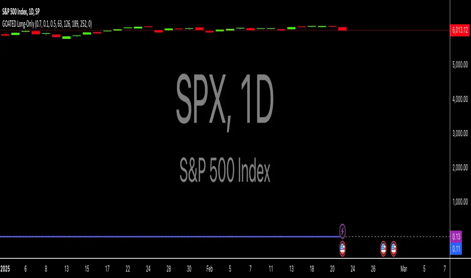
Long-Only For SPXThe "GOATED Long-Only" TradingView strategy, written in Pine Script v5, is designed for long-term momentum trading with a $50 initial capital. It identifies high-momentum stocks by calculating a composite momentum score across 3-month (63 days), 6-month (126 days), 9-month (189 days), and 12-month (252 days) periods, using the formula (current_price / past_price) - 1. The strategy filters stocks with annualized volatility below 0.5 (calculated as the standard deviation of daily returns, annualized by multiplying by the square root of 252 trading days) and requires momentum to exceed a customizable threshold (default 0.0). It enters long positions when momentum becomes positive and exits when it turns negative, using stop-loss (1%) and take-profit (50%) levels to manage risk. The strategy visualizes momentum and volatility on the chart, plotting entry/exit signals as green triangles (long entry) and red triangles (long exit) for backtesting and analysis.
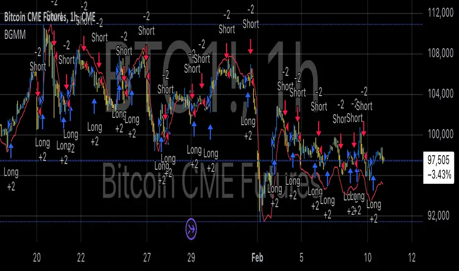
BTC Future Gamma-Weighted Momentum Model (BGMM)The BTC Future Gamma-Weighted Momentum Model (BGMM) is a quantitative trading strategy that utilizes the Gamma-weighted average price (GWAP) in conjunction with a momentum-based approach to predict price movements in the Bitcoin futures market. The model combines the concept of weighted price movements with trend identification, where the Gamma factor amplifies the weight assigned to recent prices. It leverages the idea that historical price trends and weighting mechanisms can be utilized to forecast future price behavior.
Theoretical Background:
1. Momentum in Financial Markets:
Momentum is a well-established concept in financial market theory, referring to the tendency of assets to continue moving in the same direction after initiating a trend. Any observed market return over a given time period is likely to continue in the same direction, a phenomenon known as the “momentum effect.” Deviations from a mean or trend provide potential trading opportunities, particularly in highly volatile assets like Bitcoin.
Numerous empirical studies have demonstrated that momentum strategies, based on price movements, especially those correlating long-term and short-term trends, can yield significant returns (Jegadeesh & Titman, 1993). Given Bitcoin’s volatile nature, it is an ideal candidate for momentum-based strategies.
2. Gamma-Weighted Price Strategies:
Gamma weighting is an advanced method of applying weights to price data, where past price movements are weighted by a Gamma factor. This weighting allows for the reinforcement or reduction of the influence of historical prices based on an exponential function. The Gamma factor (ranging from 0.5 to 1.5) controls how much emphasis is placed on recent data: a value closer to 1 applies an even weighting across periods, while a value closer to 0 diminishes the influence of past prices.
Gamma-based models are used in financial analysis and modeling to enhance a model’s adaptability to changing market dynamics. This weighting mechanism is particularly advantageous in volatile markets such as Bitcoin futures, as it facilitates quick adaptation to changing market conditions (Black-Scholes, 1973).
Strategy Mechanism:
The BTC Future Gamma-Weighted Momentum Model (BGMM) utilizes an adaptive weighting strategy, where the Bitcoin futures prices are weighted according to the Gamma factor to calculate the Gamma-Weighted Average Price (GWAP). The GWAP is derived as a weighted average of prices over a specific number of periods, with more weight assigned to recent periods. The calculated GWAP serves as a reference value, and trading decisions are based on whether the current market price is above or below this level.
1. Long Position Conditions:
A long position is initiated when the Bitcoin price is above the GWAP and a positive price movement is observed over the last three periods. This indicates that an upward trend is in place, and the market is likely to continue in the direction of the momentum.
2. Short Position Conditions:
A short position is initiated when the Bitcoin price is below the GWAP and a negative price movement is observed over the last three periods. This suggests that a downtrend is occurring, and a continuation of the negative price movement is expected.
Backtesting and Application to Bitcoin Futures:
The model has been tested exclusively on the Bitcoin futures market due to Bitcoin’s high volatility and strong trend behavior. These characteristics make the market particularly suitable for momentum strategies, as strong upward or downward movements are often followed by persistent trends that can be captured by a momentum-based approach.
Backtests of the BGMM on the Bitcoin futures market indicate that the model achieves above-average returns during periods of strong momentum, especially when the Gamma factor is optimized to suit the specific dynamics of the Bitcoin market. The high volatility of Bitcoin, combined with adaptive weighting, allows the model to respond quickly to price changes and maximize trading opportunities.
Scientific Citations and Sources:
• Jegadeesh, N., & Titman, S. (1993). Returns to Buying Winners and Selling Losers: Implications for Stock Market Efficiency. The Journal of Finance, 48(1), 65–91.
• Black, F., & Scholes, M. (1973). The Pricing of Options and Corporate Liabilities. Journal of Political Economy, 81(3), 637–654.
• Fama, E. F., & French, K. R. (1992). The Cross-Section of Expected Stock Returns. The Journal of Finance, 47(2), 427–465.
Engulfing Pattern with Volume and EMAs
**Strategy Overview:
This strategy combines price action (Engulfing patterns), volume analysis, trend confirmation (EMAs), and noise reduction (ATR filter) to generate high-probability trading signals.
Engulfing Pattern with Volume, EMAs, and Market Noise Filter**
This strategy identifies bullish and bearish Engulfing candlestick patterns, combined with volume analysis, moving averages (EMAs), and a market noise filter to generate trading signals.
**Key Components:**
1. **Engulfing Pattern Detection:**
- **Bullish Engulfing**: A green candle completely engulfs the previous red candle.
- **Bearish Engulfing**: A red candle completely engulfs the previous green candle.
2. **Volume Filter:**
- Signals are validated only if the current volume is higher than the 20-period Simple Moving Average (SMA) of volume.
3. **EMA Indicators:**
- Three EMAs are plotted: 50-period (blue), 89-period (orange), and 200-period (red).
- These EMAs help identify the trend direction and provide additional confirmation.
4. **Market Noise Filter:**
- Uses the Average True Range (ATR) to filter out insignificant price movements.
- A signal is considered valid only if the price movement (absolute difference between open and close) is greater than 0.5 times the 14-period ATR.
**Trading Signals:**
**Buy Signal**:
- Bullish Engulfing pattern + High volume (above SMA 20) + Significant price movement (filtered by ATR).
- Plotted as a green "BUY" label below the candle.
**Sell Signal**:
- Bearish Engulfing pattern + High volume (above SMA 20) + Significant price movement (filtered by ATR).
- Plotted as a red "SELL" label above the candle.
**Customization:**
- Users can adjust EMA lengths, volume SMA period, and ATR multiplier to suit their trading preferences.
Fibonacci Retracement/ExtensionThis Pine Script code implements Fibonacci retracement and extension levels based on a ZigZag pattern. Below is a breakdown of its functionality:
Overview
The script calculates Fibonacci retracement and extension levels by identifying swing highs and swing lows using the ZigZag algorithm. It then plots these levels on the chart for trend analysis.
1. ZigZag Length Input
Defines the ZigZag length, which determines the sensitivity of peak and trough identification.
2. Fibonacci Retracement Calculation
Computes Fibonacci retracement levels using swing highs and lows.
Uses pre-defined Fibonacci ratios (0.236, 0.382, 0.5, 0.618, 0.786, 1.0).
Adjusts line positions dynamically as the trend evolves.
3. Fibonacci Extension Calculation
Identifies Fibonacci extension levels for future price targets.
Uses previous ZigZag patterns to estimate potential price movements.
4. Trend and Fibonacci Configuration
Allows the user to configure Fibonacci trend analysis.
TrendSw: Sets the trend direction (1 = Bullish, -1 = Bearish, 0 = None).
ZigZagleg: Determines the countback value for retracement calculations.
waves█ OVERVIEW
This library intended for use in Bar Replay provides functions to generate various wave forms (sine, cosine, triangle, square) based on time and customizable parameters. Useful for testing and in creating oscillators, indicators, or visual effects.
█ FUNCTIONS
• getSineWave()
• getCosineWave()
• getTriangleWave()
• getSquareWave()
█ USAGE EXAMPLE
//@version=6
indicator("Wave Example")
import kaigouthro/waves/1
plot(waves.getSineWave(cyclesPerMinute=15))
█ NOTES
* barsPerSecond defaults to 10. Adjust this if not using 10x in Bar Replay.
* Phase shift is in degrees.
---
Library "waves"
getSineWave(cyclesPerMinute, bar, barsPerSecond, amplitude, verticalShift, phaseShift)
`getSineWave`
> Calculates a sine wave based on bar index, cycles per minute (BPM), and wave parameters.
Parameters:
cyclesPerMinute (float) : (float) The desired number of cycles per minute (BPM). Default is 30.0.
bar (int) : (int) The current bar index. Default is bar_index.
barsPerSecond (float) : (float) The number of bars per second. Default is 10.0 for Bar Replay
amplitude (float) : (float) The amplitude of the sine wave. Default is 1.0.
verticalShift (float) : (float) The vertical shift of the sine wave. Default is 0.0.
phaseShift (float) : (float) The phase shift of the sine wave in radians. Default is 0.0.
Returns: (float) The calculated sine wave value.
getCosineWave(cyclesPerMinute, bar, barsPerSecond, amplitude, verticalShift, phaseShift)
`getCosineWave`
> Calculates a cosine wave based on bar index, cycles per minute (BPM), and wave parameters.
Parameters:
cyclesPerMinute (float) : (float) The desired number of cycles per minute (BPM). Default is 30.0.
bar (int) : (int) The current bar index. Default is bar_index.
barsPerSecond (float) : (float) The number of bars per second. Default is 10.0 for Bar Replay
amplitude (float) : (float) The amplitude of the cosine wave. Default is 1.0.
verticalShift (float) : (float) The vertical shift of the cosine wave. Default is 0.0.
phaseShift (float) : (float) The phase shift of the cosine wave in radians. Default is 0.0.
Returns: (float) The calculated cosine wave value.
getTriangleWave(cyclesPerMinute, bar, barsPerSecond, amplitude, verticalShift, phaseShift)
`getTriangleWave`
> Calculates a triangle wave based on bar index, cycles per minute (BPM), and wave parameters.
Parameters:
cyclesPerMinute (float) : (float) The desired number of cycles per minute (BPM). Default is 30.0.
bar (int) : (int) The current bar index. Default is bar_index.
barsPerSecond (float) : (float) The number of bars per second. Default is 10.0 for Bar Replay
amplitude (float) : (float) The amplitude of the triangle wave. Default is 1.0.
verticalShift (float) : (float) The vertical shift of the triangle wave. Default is 0.0.
phaseShift (float) : (float) The phase shift of the triangle wave in radians. Default is 0.0.
Returns: (float) The calculated triangle wave value.
getSquareWave(cyclesPerMinute, bar, barsPerSecond, amplitude, verticalShift, dutyCycle, phaseShift)
`getSquareWave`
> Calculates a square wave based on bar index, cycles per minute (BPM), and wave parameters.
Parameters:
cyclesPerMinute (float) : (float) The desired number of cycles per minute (BPM). Default is 30.0.
bar (int) : (int) The current bar index. Default is bar_index.
barsPerSecond (float) : (float) The number of bars per second. Default is 10.0 for Bar Replay
amplitude (float) : (float) The amplitude of the square wave. Default is 1.0.
verticalShift (float) : (float) The vertical shift of the square wave. Default is 0.0.
dutyCycle (float) : (float) The duty cycle of the square wave (0.0 to 1.0). Default is 0.5 (50% duty cycle).
phaseShift (float) : (float) The phase shift of the square wave in radians. Default is 0.0.
Returns: (float) The calculated square wave value.
