IKAKOver2change point
Improve the accuracy of reverse sign
Adding a signature using only RCI
変更点
逆張りのサインと順張りのサインを区別し、逆張りのサインは騙しができるだけ少なくなるように精度を上げました。
逆張りか順張りかは10emaと100emaの位置関係だけで区別しています。
また、RCIのみを利用した、レンジ相場用のサインを追加しました。
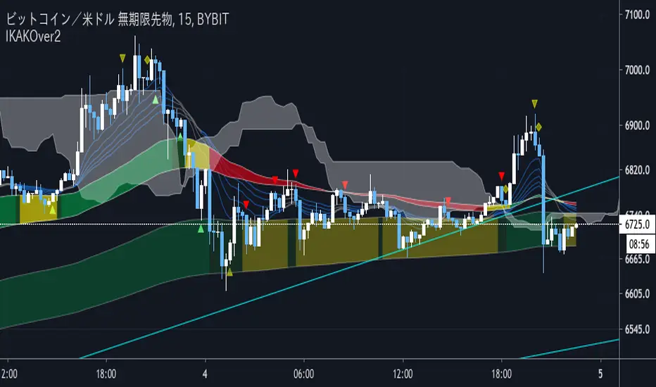
We have set a period such as EMA to use 5 minute bars and the first band is period 60 and 100 EMA . The color of the belt changes according to the position of the period 5EMA-25EMA-50EMA. The second sash is based on a 60- and 100-EMA period of 15 minutes. The change in the color of the obi is also a 15-minute specification.
Since the above period can be changed, I think that there are customs such as 1 hour and 4 hours.
Buying and selling signs are shown in green for buying and red for selling. (More frequent)
For the time being, it is also possible to display the Ichimoku balance table.
As for my usage method, when both the 15-minute and 5-minute bars have an uptrend (downtrend ), when each trading sign is confirmed, spread the limit just below the price. . (Because there is a commission in the market)
If the color of the obi becomes yellow, the trend may be over, so wait for the signature to reach the bundle of 15 minutes instead of 5 minutes, and after the signature is confirmed, it is the same as 5 minutes.
The loss cut line is often the latest low. Or when the obi is broken. .
I am still studying about profitability. Sometimes we use indicators, sometimes we reach the target horizon. I think each way is good.
It is a discretionary aid, and the head and tail are cut off, and the image is about 10 to 100 $.
Buscar en scripts para "股价站上60月线"
IKAKOWe have set a period such as EMA to use 5 minute bars and the first band is period 60 and 100 EMA. The color of the belt changes according to the position of the period 5EMA-25EMA-50EMA. The second sash is based on a 60- and 100-EMA period of 15 minutes. The change in the color of the obi is also a 15-minute specification.
Since the above period can be changed, I think that there are customs such as 1 hour and 4 hours.
Buying and selling signs are shown in green for buying and red for selling. (More frequent)
For the time being, it is also possible to display the Ichimoku balance table.
As for my usage method, when both the 15-minute and 5-minute bars have an uptrend (downtrend ), when each trading sign is confirmed, spread the limit just below the price. . (Because there is a commission in the market)
If the color of the obi becomes yellow, the trend may be over, so wait for the signature to reach the bundle of 15 minutes instead of 5 minutes, and after the signature is confirmed, it is the same as 5 minutes.
The loss cut line is often the latest low. Or when the obi is broken. .
I am still studying about profitability. Sometimes we use indicators, sometimes we reach the target horizon. I think each way is good.
It is a discretionary aid, and the head and tail are cut off, and the image is about 10 to 100 $.

High Low Cloud Strategy BacktestingHigh Low Cloud Strategy Backtesting: this is a breakout and reversal previous trend strategy
A. Indicator: row 6 to row 17
1. Fast Cloud
Upper line = ema of High with 60 periods
Lower line = ema of Low with 60 periods
1. Slow Cloud
Upper line = ema of High with 240 periods
Lower line = ema of Low with 240 periods
B. Strategy Backtesting
1. Chart IDC, Time frame: M30
2. Long condition: row 20 to row 34
a. Entry =
* Upper line of Fast Cloud below Lower line of Slow Cloud
* Price crossover Upper line of Slow Cloud
b. Stoploss =
* Price crossunder bottom of 240 periods (~ bottom of 5 days)
c. Takeprofit =
* Lower line of Fast Cloud above Upper line of Slow Cloud
* Price crossunder Lower line of Fast Cloud
3. Short condition: row 37 to row 49
a. Entry =
* Lower line of Fast Cloud above Upper line of Slow Cloud
* Price crossunder Lower line of Slow Cloud
b. Stoploss =
* Price crossover peak of 240 periods (~ bottom of 5 days)
c. Takeprofit =
* Upper line of Fast Cloud below Lower line of Slow Cloud
* Price crossover Upper line of Fast Cloud

Ichimoku [Gu5]Original Ichimoku Kinko Hyo created by Goichi Hosoda 1930
Knowing how to interpret the Ichimoku indicator can be complicated. I hope this version is more intuitive
Use Ichimoku to determine the trend of the day
When the market is above the cloud, and Tenkan (green line) crosses over Kijun (red Line), there is a Bullish Trend . When Tenkan crosses under Kijun, the trend ends.
When the market is under the cloud, and Tenkan crosses under Kijun; There is a Bearish Trend . When Tenkan crosses over Kijun, the trend ends.
When the market crosses the cloud (orange bars), there is no trend
The default setting is 9, 26 and 52. For cryptocurrencies (24/7 market), you can change it to 10, 30 and 60 periods.
///
Ichimoku Kinko Hyo fue creado por Goichi Hosoda en 1930
Saber interpretar al indicador Ichimoku puede ser complicado. Espero esta version sea mas intuitiva
Use Ichimoku para determinar la tendencia del día, y operar solo a favor de la misma
Cuando el mercado esta sobre la nube y Tenkan (linea verde) cruza sobre Kijun (linea roja), la tendencia es alcista. Cuando Tenkan cruza bajo Kijun, termina la tendencia.
Cuando el mercado esta bajo la nube y Tenkan cruza bajo Kijun, la tendencia es bajista. Cuando Tenkan cruza sobre Kijun, termina la tendencia.
Cuando el mercado atraviesa la nube (barras naranjas), no hay tendencia
Por defecto, el seteo es 9, 26 y 52. Para criptomonedas, puede cambiarlo a 10, 30 y 60 períodos

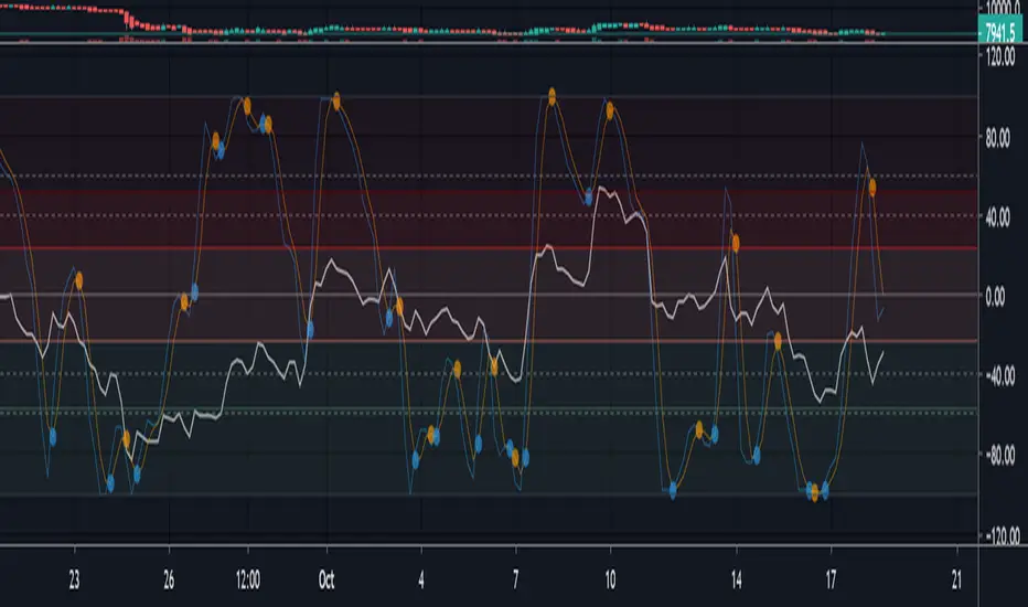
Multi momentum indicatorScript contains couple momentum oscillators all in one pane
List of indicators:
RSI
Stochastic RSI
MACD
CCI
WaveTrend by LazyBear
MFI
Default active indicators are RSI and Stochastic RSI
Other indicators are disabled by default
RSI, StochRSI and MFI are modified to be bounded to range from 100 to -100. That's why overbought is 40 and 60 instead 70 and 80 while oversold -40 and -60 instead 30 and 20.
MACD and CCI as they are not bounded to 100 or 200 range, they are limited to 100 - -100 by default when activated (extras are simply hidden) but there is an option to show full indicator.
In settings there are couple more options like show crosses or show only histogram.
Default source for all indicators is close (except WaveTrend and MFI which use hlc3) and it could be changed but for all indicators.
There is an option for 2nd RSI which can be set for any timeframe and background calculated by Fibonacci levels.
Visual RSI [LucF]Visual RSI offers a different way of looking at RSI by providing a composite representation of 9 different RSI-generated components. Instead of focusing on one line only, this approach blends multiple sources to provide the viewer with a larger context RSI-based picture.
For those who don’t want to read
• Green in bullish (>50) zone is the most bullish.
• Red in bullish zone doesn’t necessarily mean bearish—it just means bullish strength is weakening. It may be just a pause before a reprise or exhaustion signalling a reversal—impossible to tell.
• The same in inverse applies to the bearish zone (<50).
For those who want to understand
The nine components making up Visual RSI are:
• a current timeframe RSI
• a higher timeframe RSI
• the delta between these two RSI lines
• for each of these three basic components, two independent Bollinger band: one calculated for the bullish section of the scale (>50) and a separate one calculated for the lower bearish region.
Dual BBs
In my view, RSI’s position with regards to the centerline is much more important than its position in extreme areas. Why? Because the building block of RSI is the ratio of the averages of up/down moves during the RSI period. When the average of ups is greater, RSI is > 50. So while a rising signal starting from 20 let’s say, indicates that the rate of change is increasing, only when it crosses 50 can we say that sentiment balance has truly become bullish, and this information is more reliable than the signal being at a level corresponding to whatever estimate we make of what constitutes an extreme value. In my landscape, the general balance of a ratio provides more valuable information than the ratio’s exact value.
The idea behind the dual BBs is to provide independent tracking information for both halves of the indicator’s space, which I find more useful than the normal method of simply adding a multiple of the standard deviation on both sides of the mean. With dual BBs, the upper BB will never go lower than the indicator’s centerline, and the lower BB will never go higher. The upper BB focuses on upper-bound volatility when the signal is bearish, and the lower BB focuses on downside volatility when the signal is bearish.
The functions used to calculate the independent BBs are reusable on other signals if a centerline can be defined for them. A clamping percentage is implemented, so that when a BB line is hugging the centerline it clamps to it. This helps in providing earlier signals when they use the BB line states.
Providing context to RSI
What RSI measures indirectly is the balance in the rate of change—or the speed of price movement, but not its instant value, otherwise RSI would be even noisier. More precisely, RSI represents the relative strength of the up/down movement in the last n bars of RSI’s length, with 14 often used because that’s what Wilder proposed (Visual RSI’s defaults are 20 for the current timeframe and 40 for the higher timeframe). At every bar, a new value is added to the equation and an old value carrying equal weight is dropped, so a large dropped off value will have more impact on RSI’s value if the new bar’s move is small. This accounts for some of RSI’s speed in identifying exhaustion after important moves, but almost for some of its noise.
Visual RSI is the result of trying to drown RSI’s noise in the context of other informational streams, while simultaneously providing even faster information than RSI alone, by giving more visual weight to the delta between the current and higher timeframe RSI’s.
How to read Visual RSI
The default settings show all 9 basic components as green/red areas of intensities varying with their importance. The most intense colors are reserved for the delta RSI and the BBs have the lightest intensities. The individual lines of components are intentionally difficult to distinguish so that focus is first on the general picture, including the all-important six-state background, and then on the delta RSI.
One entry setup could be reversals in a larger trend context, so low pivots of the delta in a fully bullish context (a green background in the upper section of the indicator), and inversely, high pivots in a fully bearish context (a red background in the lower section of the indicator).
Please resist the common misconception, when interpreting RSI, that a reversal in the signal will necessarily lead to a reversal in price. Each trend has its rhythm. Only machine-generated price action can progress regularly. It’s normal for trends to take a breather for some time before they continue or reverse, as traders driving the trend experience emotional fatigue and gradual fear. RSI reversals merely signify that such a breather has occurred—nothing more. Only the larger context can provide information that can situate that pause and put more meaningful odds on it having more probability of continuing in one direction or the other. This is the reasoning behind the setup just described.
Features
• All components can be hidden, displayed as a simple line, a uniformly colored fill, or a green/red fill (the default).
• The background can be colored using 9 different methods, including 3 six-state methods using the rising/falling BB lines of the 3 basic components. These six states allow for bullish/bearish/neutral sentiment in both the upper and lower regions of the indicator. A bearish (dark red) background in the bullish (>50) section of the indicator represents decreasing bullishness. A bearish (slightly brighter red) in the bearish (<50) section of the indicator means incresingly bearish sentiment. The six-state backgrounds allow for neutral (no color) sentiment when no compelling signs can be found to conclude anything with meaningful odds. The default background uses the six-state method on the higher timeframe RSI’s BBs because I find it the most useful, as it represents the largest—and slowest—context sentiment among all the indicator’s components.
• A thin status bar in the top part of the indicator also allows selection of the same 9 methods to color it. The default is a triple-state system using the rising/falling characteristics of the current timeframe RSI’s BBs to provide a short-term counterbalance to the long-term background.
• Three different markers can be configured using approximately 70 permutations each, each filtered by 20 different filter permutations. When modification of the relevant parameters in the script’s Settings/Settings/Parameters section is added, possibilities are almost endless. If the generated signals are then fed into the PineCoders Engine and combined with the Engine’s own options, the permutations go up another order of magnitude, and changes to any setting can be instantly evaluated using the Engine’s backtesting results.
• Five simple filters can be combined. They are additive. They include volume-related conditions and a chandelier, which I find useful because both volume and volatility (the chandelier using highs/lows and ATR) are sensible complementary sources to RSI’s momentum information. The filter’s state can be shown as a thin line at the bottom of the indicator.
• Alerts can be configured using any of the marker/filter combinations mentioned. As usual, once your markers/filters are set up the way you want, create your alert from the chart/timeframe you want the alert to run on and be sure to use the “Once Per Bar Close” triggering condition. Use an alert message that will remind you of which combination of markers were used when creating the alert.
• A plot providing entry signals for the PineCoders Backtesting & Trading Engine is supplied. It will use whichever marker/filter configuration is active to generate signals.
• All higher timeframe information is non-repainting. Higher timeframe lines can be smoothed (the default). The selection of the higher timeframe can be made using 3 different methods:
1. By steps (if current timeframe <= 1 minute: 60 min, <= 60 min: 1D, <= 6H: 3D, <= 1D: 1W, <=1W: 1M, >1W: 12M)
2. By a user-defined multiple of the current timeframe
3. Using a fixed timeframe
Thanks to:
• Alex Orekhov aka @everget for the chandelier code.
• @RicardoSantos who through a small remark early on, unknowingly put me on the track of eliminating noise through visual crowding.
• The brilliant guys in the PineCoders Pro room for your knowledge, limitless creativity and constant companionship.
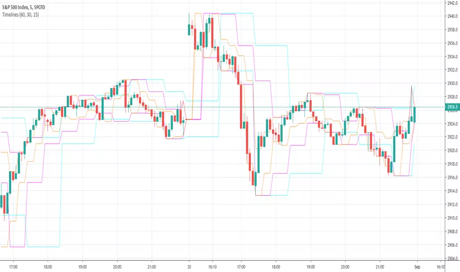
Timelines-Buschi
English:
This is a little, simple script I made upon request from a user.
It shows the highs ad lows of up to three custom timelines (e. g. 60 min, 30 min and 15 min) within a chart.
Deutsch:
Dies ist ein kleines, einfaches Skript, das ich auf Anfrage eines Nutzers erstellt habe.
Es zeigt die Hochs und Tiefs von bis zu drei individueller Zeitreihen (z. B. 60 min, 30 min und 15 min) innerhalb eines Charts.
Supertrend MTF LAG ISSUEThis script based on
we all use Super trend but it main issue is the lag as it buy too late or sell too late
using Deavaet study of Heat map MTF we can do a little trick
if you look on his study you can see that major signal for example will happen in the time frame before it happen at larger time frame
so in this example if signal at MTF 30 min and signal at MTF 60 min happen at the same time at 2 hours or 4 hours candles then this signal are more likely to be true then random signal at each time frame specific.
since we use shorter time frame on larger time frame we can remove the lag issue that make supertrend not so effective
In this example I set the signal to be MTF 30 +60 om 2 hour TF , can be good also for 4 hour candles..
So you get the signal to close inside the larger candle
now if you want to make on even shorter TF then change the code to 15 and 30 MTF on candles on 1 hour
or 1 and 5 min on 30 min or 15 min

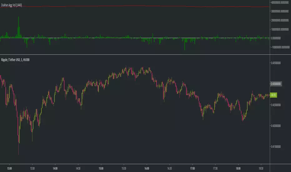
Dukhan 24 Hours rolling volume similar to exchanges Shows 24 hour rolling volume similar to the exchange - Done for BTC but works on anything
input is number of candle to calculate back
usage:
1m candle : 24h * 60 = 1440
5m candle: (24h * 60) / 5 = 288
etc
Parabolic DetectionThis method of trend analysis draws the RSI channel from 50 to 60 on the chart. If it's over 60, the channel is green.
When Bitcoin goes on its insane runs, the RSI on the 3 day chart will often be pegged at extreme values. Our goal is to visually represent these moments.
By default, this uses the 3 day resolution for its calculations. Feel free to disable this and it will work on any timeframe.

rainbow ema갤럭시님 이평선 토대로 JB가 에디트한 지수이평선 모음입니다. 편집하시면 일반 이평선으로도 사용이 가능합니다.
하나의 지표 추가 만으로 여러개의 지수이평선을 사용하실 수 있고, 제가 자주 사용하는 7,14,21,28,40,60,120,200,300선 넣어 놨습니다.
"Galaxy" made, JB edited EMA script. Editing is free for use if you swap ema to ma as a base setting.
You can use several ema lines by adding one indicator only, and I put 7,14,21,28,40,60,120,200,300 as a threshold which I frequently use.
It is made as an open source at any time possible, so that you are free for playing with it.
Gazua!!!!

TRADE.GODANN-based script, comparing the previous and current closing of the asset with its percentage of change and determining the purchase or sale accordingly.
I recommend using the time of the script in 60 minutes and the time of opration and 5 minutes for a better scalp.
For junior time I recommend 240 minutes for the script time and 60 minutes for the operating time.
Thanks Thiago Kerbes;)

RSI|The Wave PrincipleThe Wave Principle | Modified RSI
30 green | 70 red = Strong Movement (Possible Impulse)
20 cyan | 80 Yellow = Strongest Movement
Support and Resistance Level (Trend Continuation)
Uptrend= 40
Downtrend = 60
Break+Retest = BR
Div = Divergence (Change in trend)
--------------------------------------------
This indicator has been modified from original RSI to fit Wave Principle characteristics:
Uptrend Impulsive Wave over 70 RSI it changes color to red, and > 80 yellow stronger impulse | Usually means continuation, at least once more.
Downtrend Impulsive Wave under 30 RSI it changes color to green, and < 20 cyan stronger impulse | Usually means continuation, at least once more.
Once RSI reached these levels, it doesn't mean trend reversal but a correction is expected. If it shows divergence along with an Ending Diagonal, it's a confirmation for trend reversal.
In a corrective wave, levels 40-60 represents support and resistance levels where price won't go further. Indicating Corrective Waves, not as strong as Impulsives.
Prices can breakout RSI trend lines and retest from the other side before continue the new trend as also described in the Wave Principle.
--------------------------------------------

The Scale Of Sacred SoundsBased on the Sacred Sound Scale
How to use it:
This indicator is designed to capture the inferred behavior of traders and investors by using two groups of averages.
Meant for longer trades and trend indicator.
Used on any timescale as needed.
Can trade on long or short where the slow MA crosses fast Ma or where the Slow MA compresses and flips open again.
Follow the trend to the end - pot of gold at the end of the rainbow :-)
References:
Based on Daryl Guppy GMMA and
www.guppytraders.com
Read more at:
whatmusicreallyis.com
There is one tuning in which the frequencies 432, 528, 424 and 440 Hz can peacefully coexist. The scale has 32+1 pure harmonic tones and the reference frequency of 256 Hz. It comes from the Natural Ascending Series of Harmonics 32 to 64 of the 8 Hz Fundamental Tone, and represents its 6th double. I call this tuning The Scale of Sacred Sounds.
Representation using ancient Sumerian/Babylonian/Vedic math:
32; 33; 34; 35; 36; 37; 38; 39; 40; 41; 42; 43; 44; 45; 46; 47; 48; 49; 50; 51; 52; 53; 54; 55; 56; 57; 58; 59; 60; 61; 62; 63; 64
Representation using musical ratios:
1/1; 33/32; 17/16; 35/32; 9/8; 37/32; 19/16; 39/32; 5/4; 41/32; 21/16; 43/32; 11/8; 45/32; 23/16; 47/32; 3/2; 49/32; 25/16; 51/32; 13/8; 53/32; 27/16; 55/32; 7/4; 57/32; 29/16; 59/32; 15/8; 61/32; 31/16; 63/32; 2/1
The math for deriving one of the above series from the other is simple. Divide all numbers from the ancient series by the first, then simplify the fractions. Conversely, the series of ratios can be turned into the series of integers by calculating their least common denominator (the smallest whole number that is a multiple of all numbers under the fraction bar) and discarding it.
Logarithmic representation using musical constants (definition given further down):
0,000; 30,772; 60,625; 89,612; 117,783; 145,182; 171,850; 197,826; 223,144; 247,836; 271,934; 295,464; 318,454; 340,927; 362,905; 384,412; 405,465; 426,084; 446,287; 466,090; 485,508; 504,556; 523,248; 541,597; 559,616; 577,315; 594,707; 611,802; 628,609; 645,138; 661,398; 677,399; 693,147

Bitfinex Longs/Shorts Ratio AlertableThis script contains Bitfinex longs/short ratio and generates alarms with a given input .default value is 60 which means alerts when either shorts/longs reach 60:40 ratio

RSI / Stoch / SRSI / MFI / Aroon Overlay [SigmaDraconis]Combines 4 popular indicators (RSI, Stoch, SRSI, MFI) and 1 peculiar one (Aroon) in 1 for those who want to save indicators but not only.
This is an evolution of my (simpler) "RSI / Stoch / Stoch RSI (SRSI) Overlay " that you can find on my scripts.
Added bands for oversold/overbought areas (70/30 common for RSI and 80/20 for SRSI and MFI), as well as a middle 50 horizontal line.
Neutral bands around 55-45 added as well that can be hidden for less clutter. I also recommend a more transparent coloring for these since Pine script doesn't allow default transparency for horizontal lines.
By default only RSI and Stoch are activated, you can activate Aroon, MFI and SRSI on the inputs window.
Some extra notes:
* RSI, Stoch and MFI can help to strengthen one's decision as well as Aroon to predict a possible trend reversal, SRSI can show when RSI has high probability of being topped or bottomed when oversold/overbought but don't forget to look at volume and how the trend progresses that can keep SRSI above 80 or below 20 while RSI and price continues to trend, divergences are most helpful here to find possible reversal areas.
* This chart depicts some interesting divergences, as well as Stoch tops and bottoms and confluences between RSI/MFI and Stoch on some over-extended tops and bottoms that shown being good reversal zones.
RSI resistances are shown as well, failing to break above 60 or the neutral zone (this is a bearish BTC trend chart after all) or failing to gain support to break up certain levels (RSI notes a more bullish trend when consistently above 60 and more bearish below 40).
If you like it and use it to profit, please tip me below :)
Tip jars:
BTC: 15nMBiEGVrdGcu9C1h6QRcTNRvugHkqrMQ
ETH: 0xC33845946c48B61fBCbEA0367ec2238CaF2b73bc
BTS: sigma-draconis

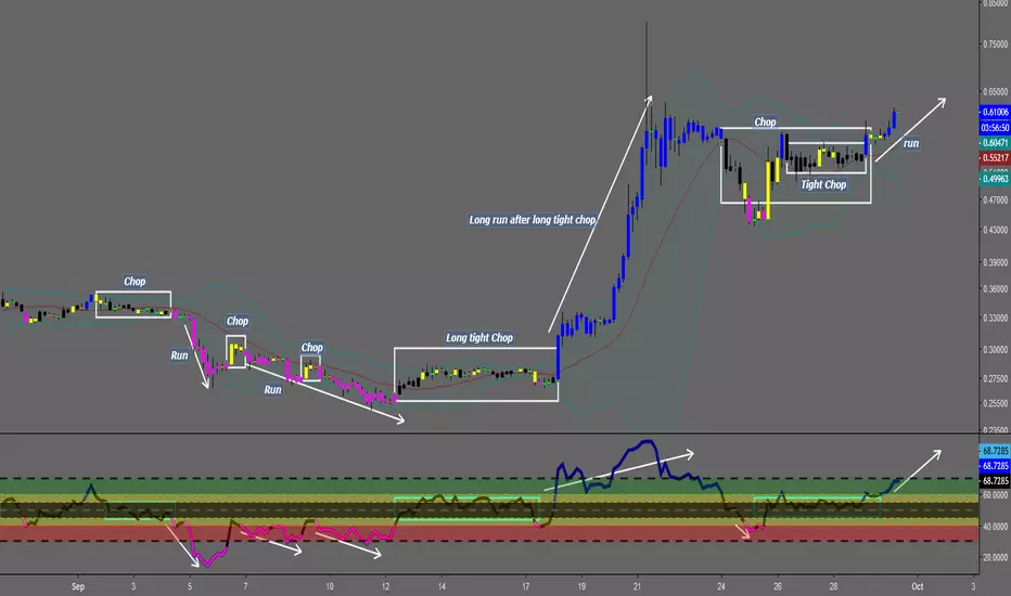
Chop and explodeThe purpose of this script is to decipher chop zones from runs/movement/explosion
The chop is RSI movement between 40 and 60
tight chop is RSI movement between 45 and 55. There should be an explosion after RSI breaks through 60 (long) or 40 (short). Tight chop bars are colored black, a series of black bars is tight consolidation and should explode imminently. The longer the chop the longer the explosion will go for. tighter the better.
Loose chop (whip saw/yellow bars) will range between 40 and 60.
the move begins with blue bars for long and purple bars for short.
Couple it with your trading system to help stay out of chop and enter when there is movement. Use with "Simple Trender."
Best of luck in all you do. Get money.
Build A BotThis is the Robot we built during the 60 Minute Build-A-Bot webinar on September 12, 2018. We had a great time, and a lot of participation and the best part was that we finished up this robot and even ran a backtest in exactly 60 minutes! We built this robot based on recommendations and suggestions from those who were attending live. Lots of pieces in this robot, but you can always tinker with it, remove stuff, add things, whatever you want!
This version uses the CCI as a trigger for trade entry. The other version uses the Hull Moving Average as a trigger for trade entry.

Volume Zone Oscillator and Price Zone (VZO/PZO) [NeoButane]" Volume Precedes Price is the conceptual idea for the oscillator."
"The main idea of the VZO was to try to change the OBV to look like an oscillator rather than an indicator, also to include time; primarily to identify which zone the volume is located in during a specific period "
How to read this indicator:
Positive reading -> bullish
Negative reading -> bearish
-60 or 60 is seen as the limit of the oscillator range, and a pullback should be expected from there.
Plus and minus signs have been added to the top and bottom for VZO and PZO, with an adjustable threshold to trigger.
Alert conditions have been added to this indicator for ease of use.
Volume Zone Oscillator, write-up by the author (recommended reading)
http:capitalsynergy.com/resources/IFTA09VZO.pdf
Volume Zone Oscillator, uses and formula
https:www.investopedia.com/articles/active-trading/072815/how-interpret-volume-zone-oscillator.asp
Price Zone Oscillator, uses and formula
https:www.investopedia.com/terms/p/price-zone-oscillator.asp

Fib,Guppy Multiple MA(FGMMA)(A/D & Volume Weight,SMA,EMA)[cI8DH]Features:
- 3 + 12 MAs (12 is chosen because Guppy has 12 MAs)
- MA types can be set to Simple, Exponential, Weighted, and Smoothed
- Volume weight can be applied to all available MAs (the built-in VWMA uses Simple MA)
- It is possible to count in only effective portions of the volume in the equation by using Accum/Dist Volume Weight
- Secondary smoothing (useful when volume weight is enabled)
- Predefined MA sets based on Fibonacci sequence (2,3,5,8,.., 377), Guppy (3,5,8,10,12,15 &30,35,40,45,50,60), and cI8DH (2,3,5,8,12,17 & 30,34,39,45,52,60)
Recommended settings:
- hlc3 as input source captures all the essential information encapsulated in a candle. I'd use hlc3 as the default option. In uptrend, "low" and in downtrend, "high" might give more relevant results when using MAs for structural analysis of a market. For commonly used MAs (EMA20, SMA50,100,200), "close" should be used due to their self-fulfilling prophecy effect.
- When you have volume weight above 0, you may want to use secondary smoothing.
- Try not to use Simple MA for smaller lengths (below 20). Sharp changes in the past (right before the period specified by the length) will affect the current value of MA dramatically leading to confusion.
- I am using the first 3 MAs for SMA 50,100,200. You can disable them from the MA type selector all at once when using Fib or Guppy ribbons.
MA-based analysis:
There are different ways of structuring a market. Geometrical (trend lines, channels, fans, patterns, etc) and Fib retracement-based structuring is very common among traders. MAs give an alternative way of analyzing markets. MA ribbons such as Guppy (6 slow and 6 fast-moving MAs) are popular for analyzing market flow. IMO default Guppy sets are a bit random as the numbers do not have an elegant sequence. So I proposed my sets based on increasing sequene spacing (+1). These two MA ribbons are good for market flow analysis but the spacing of the MAs are not ideal for structuring a market. Ribbons based on the Fib sequence is a better choice for structuring a market. This is the equivalent of Fib channels but in a more dynamic form. Among other things, MA Fib ribbon can be used to assess market momentum and to compare different stages of a market. Here are two "educational-only" examples:
Notes:
- Smoothed MA with length L = Exponential MA with length 2*L-1
- Read the background section in my ADP indicator to understand how A/D Volume is calculated

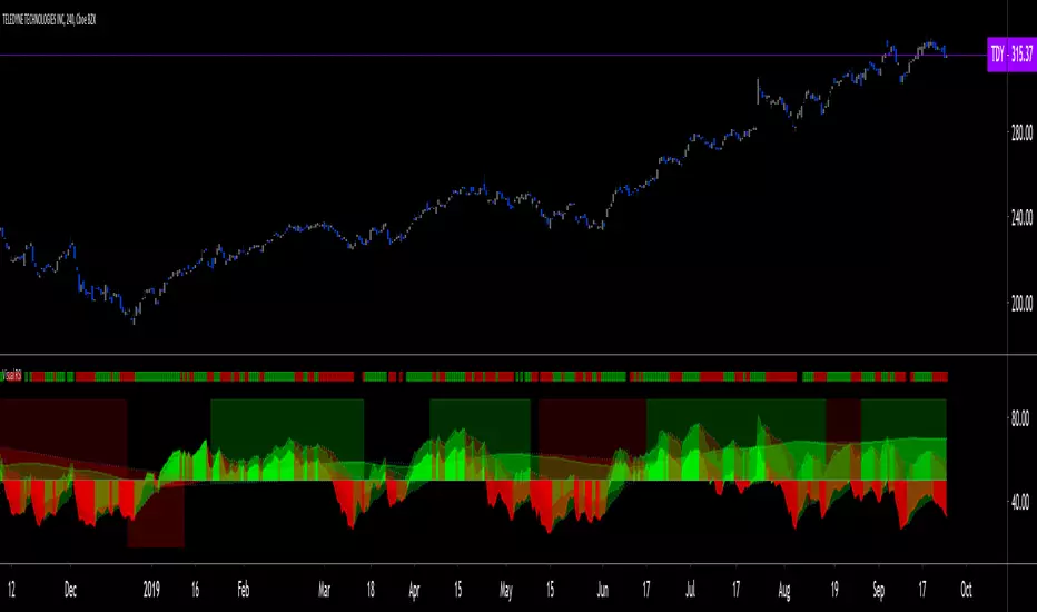
Better RSI with bullish / bearish market cycle indicator This script improves the default RSI. First. it identifies regions of the RSI which are oversold and overbought by changing the color of RSI from white to red. Second, it adds additional reference lines at 20,40,50,60, and 80 to better gauge the RSI value. Finally, the coolest feature, the middle 50 line is used to indicate which cycle the price is currently at. A green color at the 50 line indicates a bullish cycle, a red color indicators a bearish cycle, and a white color indicates a neutral cycle.
The cycles are determined using the RSI as follows:
if RSI is overbought, cycle switches to bullish until RSI falls below 40, at which point it becomes neutral
if RSI is oversold, cycle switches bearish until RSI rises above 60, at which point it becomes neutral
a neutral cycle is exited at either overbought or oversold conditions
Very useful, please give it a try and let me know what you think

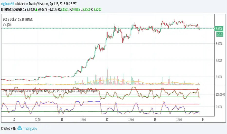
MG - Multiple time frame Stochastic RSIAllows user to view stochastic RSI from two different time frames.
Each stochastic RSI indicator is fully customizable, offering the following options:
- Timeframe
- RSI source
- RSI length
- Stochastic length
- Stochastic average length
- Stochastic smoothing length
Usage:
Comparing stochastic RSI across two different time frames can sharpen trades. For example, if you configure a 60 min and 5/15 min stochastic RSI pair, you might enter a long trade when the 60 min stoch RSI crosses up and exit / take profit when the 5 min stock RSI crosses down.
NG [Simple Harmonic Oscillator]The SHO is a bounded oscillator for the simple harmonic index that calculates the period of the market’s cycle.
The oscillator is used for short and intermediate terms and moves within a range of -100 to 100 percent.
The SHO has overbought and oversold levels at +40 and -40, respectively.
At extreme periods, the oscillator may reach the levels of +60 and -60.
The zero level demonstrates an equilibrium between the periods of bulls and bears.
The SHO oscillates between +40 and -40.
The crossover at those levels creates buy and sell signals.
In an uptrend, the SHO fluctuates between 0 and +40 where the bulls are controlling the market.
On the contrary, the SHO fluctuates between 0 and -40 during downtrends where the bears controlthe market.
Reaching the extreme level -60 in an uptrend is a sign of weakness.
