Quant Stats: Alpha, Beta, R2Quant Stats Indicator for TradingView: Alpha, Beta, and R-Squared
Overview
The Quant Stats Indicator is a professional-grade Pine Script tool designed for quantitative traders and hedge fund managers who need real-time analysis of stock or ETF performance against a benchmark using three fundamental CAPM metrics: Beta, R-Squared, and Alpha.
This indicator calculates three critical measurements that answer every quant trader's core questions: How volatile is this asset relative to my benchmark? How much of its performance is independent of the benchmark? And how much excess return am I achieving after adjusting for risk?
The Three Metrics Explained
Beta (β) measures systematic risk and volatility relative to your chosen benchmark. A Beta of 1.0 means the asset moves in lockstep with the benchmark. A Beta above 1.0 indicates higher volatility—if the market rises 10%, a Beta-1.5 asset should rise 15%. Conversely, a Beta below 1.0 indicates lower volatility, making it a defensive position. This metric helps you understand how much market exposure you're truly taking.
R-Squared (R²) quantifies what percentage of an asset's price movement can be explained by benchmark movements. An R² of 0.95 means 95% of the asset's moves are driven by the benchmark, leaving only 5% unexplained. Conversely, an R² of 0.2 means 80% of the asset's movement is independent of the benchmark. This distinction is crucial: high R² is desirable for passive index tracking but indicates weak alpha potential; low R² reveals genuine independent returns, exactly what active managers seek.
Alpha (α) reveals Jensen's Alpha—the excess risk-adjusted return after accounting for the return you "should" earn given your Beta exposure. A positive Alpha of 15% means you're outperforming the market by 15 percentage points after adjusting for systematic risk. This is the holy grail of stock picking: pure skill-driven excess return, not luck from market exposure.
How to Use It
Configure four key inputs: your benchmark ticker (default SPY, but use QQQ for tech-focused analysis or sector-specific ETFs), the lookback period in days, and the risk-free rate reflecting current Treasury yields. The lookback period is critical. Use 20 days for tactical trading to capture short-term sentiment and beta spikes; use 63 days for swing trading and quarterly rebalancing; use 252 days for structural asset allocation decisions.
The indicator plots Beta as a blue line, R-Squared as a red shaded background area, and Alpha as a green line in a sub-panel. Reference gridlines appear at Beta = 1.0 (market-equivalent volatility) and Alpha = 0.0 (breakeven performance), making interpretation intuitive.
Practical Applications
For swing traders monitoring a 63-day window, seek positions with low Beta (below 0.8) and positive Alpha—these are defensive winners. Avoid high Beta (above 1.2) with low R² unless you specifically want high-volatility speculation. Long/short hedge funds should use a 20-day lookback to detect regime changes: sudden Beta spikes often precede correlation breakdowns, while R² collapses signal rising idiosyncratic risk requiring immediate rebalancing.
For ETF portfolio construction, high R² (above 0.95) indicates index-tracking that doesn't justify active management fees. Low R² (below 0.3) combined with positive Alpha reveals genuine active management skill. The sweet spot is moderate Beta (0.5–0.8) with low R² and positive Alpha—a true diversifier that reduces portfolio volatility while generating independent returns.
Critical Interpretation Rules
A common mistake is assuming high R² is always desirable. It isn't. Passive index funds naturally have high R²; active managers should target low R² with high Alpha. Similarly, don't assume Alpha above 10% is sustainable—short-term Alpha (20–100 days) is inherently volatile and often represents temporary mispricings rather than repeatable skill. Always pair Beta analysis with R² interpretation; Beta alone ignores idiosyncratic risk, liquidity constraints, and tail risk.
Configuration Recommendations
Conservative investors should use SPY as benchmark with a 252-day lookback, targeting Alpha above 3% and Beta below 0.8. Growth-oriented portfolios might use QQQ with a 63-day lookback, targeting 8–12% Alpha and tolerating Beta up to 1.3. Hedge funds pursuing market-neutral strategies should use SPY with a 20-day lookback, set the risk-free rate to 2% (anticipating rate cuts), and target 15%+ Alpha while maintaining Beta below 0.3.
Important Limitations
The indicator is backward-looking; historical statistical relationships may not persist. Shorter lookback periods are noisier but more responsive; longer periods smooth noise but lag regime changes. Choosing the wrong benchmark completely invalidates analysis. Finally, the indicator doesn't account for tail risk or extreme market events where correlations spike unpredictably and Beta becomes unreliable.
Use this tool to separate signal from noise and identify true alpha generators. Apply it consistently, validate results against official fund factsheets, and monitor for 2–4 weeks before making significant portfolio decisions.
R2

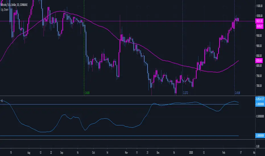
r2 correlation coefficientmade a quick script to compare r2 correlation coefficient, can change source and correlation component in inputs menu
example, here we can see that btc currently has a 0.85 correlation with eth vs usd when using simple moving avg on the daily (above 0.8 is positive correlation. below -0.8 is negitive correlation, and anything in between means there is no correlation)
note: if you wanted to compare with a different source like rsi, then you would need to reduce the length in the inputs menu
not an expert, i encourage doing your own research
biffy
R2-Adaptive RegressionIntroduction
I already mentioned various problems associated with the lsma, one of them being overshoots, so here i propose to use an lsma using a developed and adaptive form of 1st order polynomial to provide several improvements to the lsma. This indicator will adapt to various coefficient of determinations while also using various recursions.
More In Depth
A 1st order polynomial is in the form : y = ax + b , our indicator however will use : y = a*x + a1*x1 + (1 - (a + a1))*y , where a is the coefficient of determination of a simple lsma and a1 the coefficient of determination of an lsma who try to best fit y to the price.
In some cases the coefficient of determination or r-squared is simply the squared correlation between the input and the lsma. The r-squared can tell you if something is trending or not because its the correlation between the rough price containing noise and an estimate of the trend (lsma) . Therefore the filter give more weight to x or x1 based on their respective r-squared, when both r-squared is low the filter give more weight to its precedent output value.
Comparison
lsma and R2 with both length = 100
The result of the R2 is rougher, faster, have less overshoot than the lsma and also adapt to market conditions.
Longer/Shorter terms period can increase the error compared to the lsma because of the R2 trying to adapt to the r-squared. The R2 can also provide good fits when there is an edge, this is due to the part where the lsma fit the filter output to the input (y2)
Conclusion
I presented a new kind of lsma that adapt itself to various coefficient of determination. The indicator can reduce the sum of squares because of its ability to reduce overshoot as well as remaining stationary when price is not trending. It can be interesting to apply exponential averaging with various smoothing constant as long as you use : (1- (alpha+alpha1)) at the end.
Thanks for reading

Chande Kroll R-Squared IndexChande Kroll R-Squared Index script.
This indicator was originally developed by Tushar S. Chande and Stanley Kroll (see their book `The New Technical Trader`, Chapter 2: `Linear Regression Analysis`).
