Kernel-regression — Indicadores y estrategias

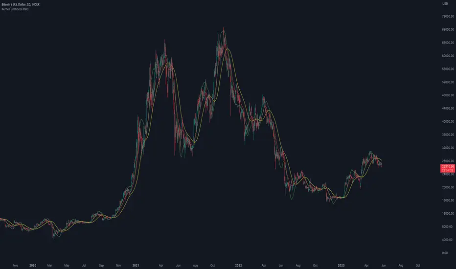
Kernel Regression Toolkit This toolkit provides filters and extra functionality for non-repainting Nadaraya-Watson estimator implementations made by @jdehorty. For the sake of ease I have nicknamed it "kreg". Filters include a smoothing formula and zero lag formula. The purpose of this script is to help traders test, experiment and develop different regression lines. Regression lines are best used as trend lines and can be an invaluable asset for quickly locating first pullbacks and breaks of trends. Other features include two J lines and a blend line. J lines are featured in tools like Stochastic KDJ. The formula uses the distance between K and D lines to make the J line. The blend line adds the ability to blend two lines together. This can be useful for several tasks including finding a center/median line between two lines or for blending in the characteristics of a different line. Default is set to 50 which is a 50% blend of the two lines. This can be increased and decreased to taste. This tool can be overlaid on the chart or on top of another indicator if you set the source. It can even be moved into its own window to create a unique oscillator based on whatever sources you feed it. Below are the standard settings for the kernel estimation as documented by @jdehorty: Lookback Window: The number of bars used for the estimation. This is a sliding value that represents the most recent historical bars. Recommended range: 3-50 Weighting: Relative weighting of time frames. As this value approaches zero, the longer time frames will exert more influence on the estimation. As this value approaches infinity, the behavior of the Rational Quadratic Kernel will become identical to the Gaussian kernel. Recommended range: 0.25-25 Level: Bar index on which to start regression. Controls how tightly fit the kernel estimate is to the data. Smaller values are a tighter fit. Larger values are a looser fit. Recommended range: 2-25 Lag: Lag for crossover detection. Lower values result in earlier crossovers. Recommended range: 1-2 For more information on this technique refer to to the original open source indicator by @jdehorty located here:

KernelFunctionsFilters Library "KernelFunctionsFilters" This library provides filters for non-repainting kernel functions for Nadaraya-Watson estimator implementations made by @jdehorty. Filters include a smoothing formula and zero lag formula. You can find examples in the code. For more information check out the original library KernelFunctions. rationalQuadratic(_src, _lookback, _relativeWeight, startAtBar, _filter) Parameters: _src (float) _lookback (simple int) _relativeWeight (simple float) startAtBar (simple int) _filter (simple string) gaussian(_src, _lookback, startAtBar, _filter) Parameters: _src (float) _lookback (simple int) startAtBar (simple int) _filter (simple string) periodic(_src, _lookback, _period, startAtBar, _filter) Parameters: _src (float) _lookback (simple int) _period (simple int) startAtBar (simple int) _filter (simple string) locallyPeriodic(_src, _lookback, _period, startAtBar, _filter) Parameters: _src (float) _lookback (simple int) _period (simple int) startAtBar (simple int) _filter (simple string) j(line1, line2) Parameters: line1 (float) line2 (float)

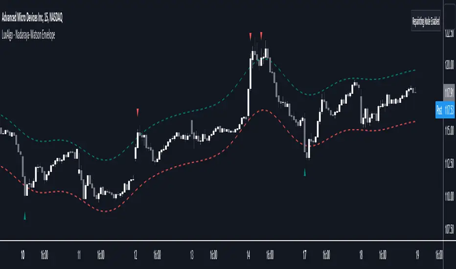
Nadaraya-Watson Envelope [LuxAlgo]This indicator builds upon the previously posted Nadaraya-Watson smoothers. Here we have created an envelope indicator based on Kernel Smoothing with integrated alerts from crosses between the price and envelope extremities. Unlike the Nadaraya-Watson estimator, this indicator follows a contrarian methodology. Please note that by default this indicator can be subject to repainting. Users can use a non-repainting smoothing method available from the settings. The triangle labels are designed so that the indicator remains useful in real-time applications. 🔶 USAGE 🔹 Non Repainting This tool can outline extremes made by the prices. This is achieved by estimating the underlying trend in the price, then calculating the mean absolute deviations from it, the obtained result is added/subtracted to the estimated underlying trend. The non-repainting method estimates the underlying trend in price using an "endpoint Nadaraya-Watson estimator", and would return similar results to more classical band indicators. 🔹 Repainting The repainting method makes use of the Nadaraya-Watson estimator to estimate the underlying trend in the price. The construction of the band extremities is the same as in the non-repainting method. We can expect the price to reverse when crossing one of the envelope extremities. Crosses between the price and the envelopes extremities are indicated with triangles on the chart. For real-time applications, triangles are always displayed when a cross occurs and remain displayed at the location it first appeared even if the cross is no longer visible after a recalculation of the envelope. By popular demand, we have integrated alerts for this indicator from the crosses between the price and the envelope extremities. However, we do not recommend this precise method to be used alone or for solely real-time applications. We do not have data supporting the performance of this tool over more classical bands/envelope/channels indicators. 🔶 SETTINGS Bandwidth: Controls the degree of smoothness of the envelopes, with higher values returning smoother results. Mult: Controls the envelope width. Source: Input source of the indicator. Repainting Smoothing: Determine if a repainting or non-repainting method should be used for the calculation of the indicator. 🔶 RELATED SCRIPTS For more information on the Nadaraya-Watson estimator see:

Nadaraya-Watson Smoothers [LuxAlgo]The following tool smoothes the price data using various methods derived from the Nadaraya-Watson estimator, a simple Kernel regression method. This method makes use of the Gaussian kernel as a weighting function. Users have the option to use a non-repainting as well as a repainting method, see the USAGE section for more information. 🔶 USAGE 🔹 Non Repainting When Repainting Smoothing is disabled the returned indicator acts similarly to a regular causal moving average. This result could be described as an "endpoint Nadaraya-Watson estimator". Unlike a regular moving average whose degree of smoothness is commonly determined by the length of its calculation window, the degree of smoothness of the proposed indicator is determined by the bandwidth setting, with a higher value returning smoother results. In the above chart, a bandwidth value of 50 is used. An increasing value of the smoother is indicative of an uptrend, while a decreasing value is indicative of a downtrend. 🔹 Repainting Non-causal smoothing methods have found low support from technical analysts because they tend to repaint. Yet, they can provide powerful insights such as estimating underlying trends in the price as well as seeing how far prices deviate from them. They can also make drawing certain patterns easier and can help see underlying structures in the price more clearly. Using higher bandwidth values allows for estimating longer-term trends in the price. Triangular labels highlight points where the direction of the estimator change. This allows for the identification of tops and bottoms in the underlying trend which can be compared to the actual price tops and bottoms. Note that multiple labels can appear in real time, highlighting real-time changes in the estimator's direction. The most recent label on a series of labels is the first to appear. This can eventually be useful for the real-time predictive application of the estimator. However, it is not a usage we particularly recommend. 🔶 DETAILS The Nadaraya-Watson estimator can be described as a series of weighted averages using a specific normalized kernel as a weighting function. For each point of the estimator at time t , the peak of the kernel is located at time t , as such the highest weights are attributed to values neighboring the price located at time t . A lower bandwidth value would contribute toward a more important weighting of the price at a precise point and would as such less smooth results. In the case where our bandwidth is so small that the resulting kernel is just an impulse, we would get the raw price back. However, when the bandwidth is sufficiently large, prices would be weighted similarly, thus resulting in a result closer to the price mean. It can be interesting to note that due to the nature of the estimator and its weighting procedure, real-time results would not deviate drastically for points in the estimator near the center of the calculation window. 🔶 SETTINGS Bandwidth : controls the bandwidth of the Gaussian kernel, with higher values returning smoother results. Src : Input source of the kernel regression. Repainting Smoothing : Determine if the smoothing method should repaint or not. If disabled the "endpoint Nadaraya-Watson estimator" is returned.