30min First Candle + Fibo50 + Sequential Multi-TF Break StrategyPrice action basée sur ouverture marché US a partir de la 1ere bougie
Réinitialisation chaque jour
Price action based on US market opening from 1st candle
Reset every day.
Análisis fundamental

30min First Candle + Fibo50 + Sequential Multi-TF Break StrategyPrice action basée sur ouverture marché US avec Réinitialisation chaque jour
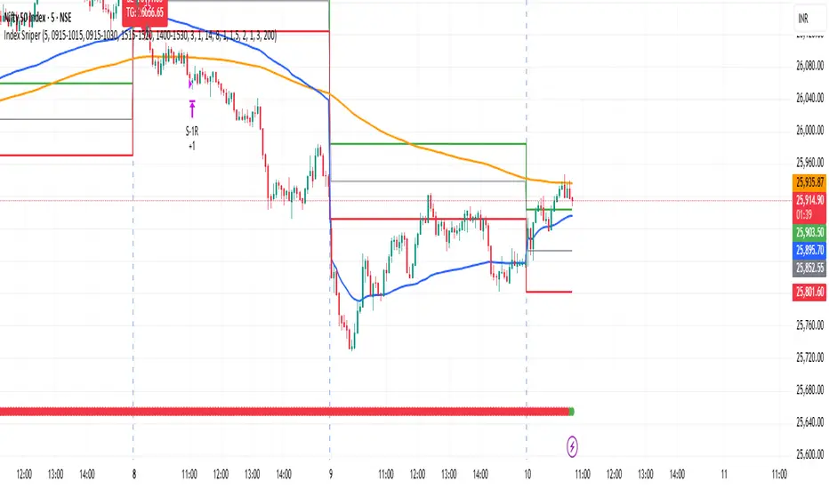
Index SniperTrade smart, trade sharp! Index Sniper Strategy targets the strongest market moves with surgical entries and strict risk control — designed for traders who want speed, confidence, and consistency in index trading.
VWolf – Hulk StrikeOVERVIEW
VWolf – Hullk Strike is a dynamic trend-following strategy designed to capture pullbacks within established moves. It combines a configurable Moving Average (HULL, EMA, SMA, or DEMA) trend filter with DMI/ADX confirmation and a Stochastic RSI timing trigger. Risk is managed through ATR- or Supertrend-based stops, optional partial profit-taking, and automatic stop adjustments. The strategy aims to rejoin momentum after controlled retracements while maintaining consistent, quantified risk
RECOMMENDED USE
Markets: Liquid indices, major FX pairs, large-cap equities, high-liquidity crypto pairs.
Timeframes: M15 to D1 (stricter filters for lower timeframes, looser for higher).
Profiles: Traders seeking structured trend participation with systematic timing.
Strengths
Highly flexible trend engine adaptable to multiple markets.
Dual confirmation reduces false signals during pullbacks.
Risk-first design with multiple stop models and partial exits.
Precautions
Over-filtering may reduce trade frequency and miss fast continuations.
Under-filtering may increase whipsaw risk in choppy markets.
Backtest vs forward-test differences if date/session filters are inconsistent.
CONCLUSION
VWolf – Hullk Strike is designed to capture the “second leg” of a trend after a controlled retracement. With configurable MA strictness, DMI/ADX strength filters, and precise Stoch RSI timing, it enhances selectivity while keeping responsiveness. Its stop/target framework—anchored stops, proportional targets, partial exits, and dynamic stop moves—offers disciplined risk control and upside preservation.
FOR MORE INFORMATION VISIT vwolftrading.com

S&D Light+ Enhanced# S&D Light+ Enhanced - Supply & Demand Zone Trading Strategy
## 📊 Overview
**S&D Light+ Enhanced** is an advanced Supply and Demand zone identification and trading strategy that combines institutional order flow concepts with smart money techniques. This strategy automatically identifies high-probability reversal zones based on Break of Structure (BOS), momentum analysis, and first retest principles.
## 🎯 Key Features
### Smart Zone Detection
- **Automatic Supply & Demand Zone Identification** - Detects institutional zones where price is likely to react
- **Multi-Candle Momentum Analysis** - Validates zones with configurable momentum requirements
- **Break of Structure (BOS) Confirmation** - Ensures zones are created only after significant structure breaks
- **Quality Filters** - Minimum zone size and ATR-based filtering to eliminate weak zones
### Advanced Zone Management
- **Customizable Zone Display** - Choose between Geometric or Volume-Weighted midlines
- **First Retest Logic** - Option to trade only the first touch of each zone for higher probability setups
- **Zone Capacity Control** - Maintains a clean chart by limiting stored zones per type
- **Visual Zone Status** - Automatically marks consumed zones with faded midlines
### Risk Management
- **Dynamic Stop Loss** - Positioned beyond zone boundaries with adjustable buffer
- **Risk-Reward Ratio Control** - Customizable R:R for consistent risk management
- **Entry Spacing** - Minimum bars between signals prevents overtrading
- **Position Sizing** - Built-in percentage of equity allocation
## 🔧 How It Works
### Zone Creation Logic
**Supply Zones (Selling Pressure):**
1. Strong momentum downward movement (configurable body-to-range ratio)
2. Identified bullish base candle (where institutions accumulated shorts)
3. Break of Structure downward (price breaks below recent swing low)
4. Zone created at the base candle's high/low range
**Demand Zones (Buying Pressure):**
1. Strong momentum upward movement
2. Identified bearish base candle (where institutions accumulated longs)
3. Break of Structure upward (price breaks above recent swing high)
4. Zone created at the base candle's high/low range
### Entry Conditions
**Long Entry:**
- Price retests a demand zone (touches top of zone)
- Rejection confirmed (close above zone)
- Zone hasn't been used (if "first retest only" enabled)
- Minimum bars since last entry respected
**Short Entry:**
- Price retests a supply zone (touches bottom of zone)
- Rejection confirmed (close below zone)
- Zone hasn't been used (if "first retest only" enabled)
- Minimum bars since last entry respected
## ⚙️ Customizable Parameters
### Display Settings
- **Show Zones** - Toggle zone visualization on/off
- **Max Stored Zones** - Control number of active zones (1-50 per type)
- **Color Customization** - Adjust supply/demand colors and transparency
### Zone Quality Filters
- **Momentum Body Fraction** - Minimum body size for momentum candles (0.1-0.9)
- **Min Momentum Candles** - Number of consecutive momentum candles required (1-5)
- **Big Candle Body Fraction** - Alternative single-candle momentum threshold (0.5-0.95)
- **Min Zone Size %** - Minimum zone height as percentage of price (0.01-5.0%)
### BOS Configuration
- **Swing Length** - Lookback period for structure identification (3-20)
- **ATR Length** - Period for volatility measurement (1-50)
- **BOS Required Break** - ATR multiplier for valid structure break (0.1-3.0)
### Midline Options
- **None** - No midline displayed
- **Geometric** - Simple average of zone top/bottom
- **CenterVolume** - Volume-weighted center based on highest volume bar in window
### Risk Management
- **SL Buffer %** - Additional space beyond zone boundary (0-5%)
- **Take Profit RR** - Risk-reward ratio for target placement (0.5-10x)
### Entry Rules
- **Only 1st Retest per Zone** - Trade zones only once for higher quality
- **Min Bars Between Entries** - Prevent overtrading (1-20 bars)
## 📈 Recommended Settings
### Conservative (Lower Frequency, Higher Quality)
```
Momentum Body Fraction: 0.30
Min Momentum Candles: 2-3
BOS Required Break: 0.8-1.0
Min Zone Size: 0.15-0.20%
Only 1st Retest: Enabled
```
### Balanced (Default)
```
Momentum Body Fraction: 0.28
Min Momentum Candles: 2
BOS Required Break: 0.7
Min Zone Size: 0.12%
Only 1st Retest: Enabled
```
### Aggressive (Higher Frequency, More Signals)
```
Momentum Body Fraction: 0.20-0.25
Min Momentum Candles: 1-2
BOS Required Break: 0.4-0.5
Min Zone Size: 0.08-0.10%
Only 1st Retest: Disabled
```
## 🎨 Visual Elements
- **Red Boxes** - Supply zones (potential selling areas)
- **Green Boxes** - Demand zones (potential buying areas)
- **Dotted Midlines** - Center of each zone (fades when zone is used)
- **Debug Triangles** - Shows when zone creation conditions are met
- Red triangle down = Supply zone created
- Green triangle up = Demand zone created
## 📊 Best Practices
1. **Use on Higher Timeframes** - 1H, 4H, and Daily charts work best for institutional zones
2. **Combine with Trend** - Trade zones in direction of overall market structure
3. **Wait for Confirmation** - Don't enter immediately at zone touch; wait for rejection
4. **Adjust for Market Volatility** - Increase BOS multiplier in choppy markets
5. **Monitor Zone Quality** - Fresh zones typically have higher success rates
6. **Backtest Your Settings** - Optimize parameters for your specific market and timeframe
## ⚠️ Risk Disclaimer
This strategy is for educational and informational purposes only. Past performance does not guarantee future results. Always:
- Use proper position sizing
- Set appropriate stop losses
- Test thoroughly before live trading
- Consider market conditions and overall trend
- Never risk more than you can afford to lose
## 🔍 Data Window Information
The strategy provides real-time metrics visible in the data window:
- Supply Zones Count
- Demand Zones Count
- ATR Value
- Momentum Signals (Up/Down)
- BOS Signals (Up/Down)
## 📝 Version History
**v1.0 - Enhanced Edition**
- Improved BOS detection logic
- Extended base candle search range
- Added comprehensive input validation
- Enhanced visual feedback system
- Robust array bounds checking
- Debug signals for troubleshooting
## 💡 Tips for Optimization
- **Trending Markets**: Lower momentum requirements, tighter BOS filters
- **Ranging Markets**: Increase zone size minimum, enable first retest only
- **Volatile Assets**: Increase ATR multiplier and SL buffer
- **Lower Timeframes**: Reduce swing length, increase min bars between entries
- **Higher Timeframes**: Increase swing length, relax momentum requirements
---
**Created with focus on institutional order flow, smart money concepts, and practical risk management.**
*Happy Trading! 📈*

D.Y Volume Swing Strategy📌 Summary of the Daniel.Yer Volume Strategy
This strategy is based on identifying the "opening volume peak" at the start of each trading day, using a user-defined sampling window.
After the sampling period ends, the strategy looks for breakouts above the daily high or below the daily low, provided they occur with a strong high-volume candle that meets the user-set threshold.
When a breakout appears in one direction, the strategy waits for an opposite-direction confirmation candle (Reversal Confirmation) and then enters a smart counter-breakout trade.
Each trade includes dynamic Stop-Loss and Take-Profit levels calculated from recent price structure, with the option to multiply stop distance according to user preference.
The strategy also gives full control over entering long only, short only, or both, as well as choosing whether trades occur exclusively from the high/low or without restrictions.
The strategy can be tested on any timeframe and evaluated across four trading directions:
✔ Buy from High
✔ Sell from High
✔ Buy from Low
✔ Sell from Low

Titan EMA Liquidity [Stansbooth]
🔥 Precision EMA + FVG Liquidity Sweep System
Advanced Buy/Sell Signal Engine for High-Probability Trade Entries
Unlock a new level of precision with this all-in-one market structure indicator built for traders who demand accuracy, clarity, and confidence.
This tool combines EMA trend filtration , Fair Value Gap (FVG) detection , and liquidity sweep analysis to deliver powerful buy and sell signals that align with institutional price behavior.
✅ Key Features
Dynamic EMA Trend Filter:
Identifies true trend direction and filters out low-quality trades. Signals only trigger when momentum aligns with higher-timeframe directional bias.
Smart FVG Detection:
Automatically highlights bullish and bearish Fair Value Gaps, helping you spot premium/discount zones where institutional traders seek entries.
Liquidity Sweep Identification:
Detects equal highs/lows, stop hunts, and engineered liquidity grabs—then confirms reversals when price sweeps liquidity and returns inside structure.
High-Accuracy Signal Engine:
Buy/Sell alerts trigger only when three layers agree:
1. EMA trend alignment
2. FVG confirmation
3. Liquidity sweep completion
This results in cleaner signals , fewer false entries, and strong trend continuation setups.
Optimized for All Market Conditions:
Works for scalping, day trading, and swing trading across Forex, Crypto, Indices, and Stocks.
What This Indicator Helps You Achieve
Capture smart-money style entries with reduced drawdown
Enter after liquidity grabs instead of before them
Avoid chop with EMA-filtered market direction
Spot precision premium/discount zones using automatic FVG mapping
Obtain high-confidence Buy/Sell signals based on institutional concept
Why Traders Love It
This system isn’t just another signal generator—it’s a market-structure aware model that reads the chart the same way professional traders do.
Every signal is based on probability stacking , giving you the clarity and confidence to take the best setups while ignoring noise.

1M XAU Cumulative Delta Volume with OB Breakouts
### Overview
This is a **session-based CVD strategy** built around the **00:00–07:00 CEST range**. It finds the high/low of that session, turns them into **adaptive ATR-based support (yellow)** and **resistance (purple)** zones, and trades only **CVD-confirmed reversals** off those levels.
---
### How it Works
* For each day, the script:
* Builds a 00:00–07:00 CEST **profile high/low**.
* Creates a **support zone** around the session low and a **resistance zone** around the session high.
* Using lower timeframe data, it reconstructs **Cumulative Volume Delta (CVD)** and a **recent delta** filter.
* It arms “pending” states when price **enters a zone from the correct side**, then confirms:
* **BUY (long):** price reclaims above support and recent CVD is strongly positive.
* **SELL (short):** price rejects below resistance and recent CVD is strongly negative.
Only these two CVD signals (`buySignal` / `sellSignal`) open trades.
---
### Strategy Logic
* **Entries**
* `buySignal` → open **long** (if flat).
* `sellSignal` → open **short** (if flat).
* No pyramiding; one position at a time.
* **Exits (only TP & SL)**
* Long: TP at `avg_price * (0.5 + TP%)`, SL at `avg_price * (1 – SL%)`.
* Short: TP at `avg_price * (0.5 – TP%)`, SL at `avg_price * (1 + SL%)`.
* No opposite-signal exits.
---
### Extras
* **Reversal markers** on yellow/purple zones and **breakout/retest markers** are plotted for context and alerts but **do not trigger entries**.
* Zone width and “thickening” are ATR-based so important touches and near-touches are easy to see.
* Only suited for **1m intraday scalping** (e.g. XAU/USD), but can be tested on other markets/timeframes.

Best strategy for scalpingThis is a next-generation Machine Learning–powered trading strategy designed for high-accuracy intraday and swing trading. It combines adaptive trend filters, probability-weighted entries, and dynamic SL/TP logic to deliver consistent, noise-free signals.
No repainting.
Customizable risk settings.
Built for serious traders who want stable performance with low drawdown.
Invite-only access only.
Pivot Fib 4H — EAStrategy uses the pivot standard to open position, it has well define entry and exit point with SL, it also has a proper money management plan, maximum 4 trades a day, each trade risk 0.5% of the account, I have it EA version of it also.

Liquidity Sweep + BOS Retest System — Prop Firm Edition🟦 Liquidity Sweep + BOS Retest System — Prop Firm Edition
A High-Probability Smart Money Strategy Built for NQ, ES, and Funding Accounts
🚀 Overview
The Liquidity Sweep + BOS Retest System (Prop Firm Edition) is a precision-engineered SMC strategy built specifically for prop firm traders. It mirrors institutional liquidity behavior and combines it with strict account-safe entry rules to help traders pass and maintain funding accounts with consistency.
Unlike typical indicators, this system waits for three confirmations — liquidity sweep, displacement, and a clean retest — before executing any trade. Every component is optimized for low drawdown, high R:R, and prop-firm-approved risk management.
Whether you’re trading Apex, TakeProfitTrader, FFF, or OneUp Trader, this system gives you a powerful mechanical framework that keeps you within rules while identifying the market’s highest-probability reversal zones.
🔥 Key Features
1. Liquidity Sweep Detection (Stop Hunt Logic)
Automatically identifies when price clears a previous swing high/low with a sweep confirmation candle.
✔ Filters noise
✔ Eliminates early entries
✔ Locks onto true liquidity grabs
2. Automatic Break of Structure (BOS) Confirmation
Price must show true displacement by breaking structure opposite the sweep direction.
✔ Confirms momentum shift
✔ Removes fake reversals
✔ Ensures institutional intent
3. Precision Retest Entry Model
The strategy enters only when price retests the BOS level at premium/discount pricing.
✔ Zero chasing
✔ Extremely tight stop loss placement
✔ Prop-firm-friendly controlled risk
4. Built-In Risk & Trade Management
SL set at swept liquidity
TP set by user-defined R:R multiplier
Optional session filter (NY Open by default)
One trade at a time (no pyramiding)
Automatically resets logic after each trade
This prevents overtrading — the #1 cause of evaluation and account breaches.
5. Designed for Prop Firm Futures Trading
This script is optimized for:
Trailing/static drawdown accounts
Micro contract precision
Funding evaluations
Low-risk, high-probability setups
Structured, rule-based execution
It reduces randomness and emotional trading by automating the highest-quality SMC sequence.
🎯 The Trading Model Behind the System
Step 1 — Liquidity Sweep
Price must take out a recent high/low and close back inside structure.
This confirms stop-hunting behavior and marks the beginning of a potential reversal.
Step 2 — BOS (Break of Structure)
Price must break the opposite side swing with a displacement candle. This validates a directional shift.
Step 3 — Retest Entry
The system waits for price to retrace into the BOS level and signal continuation.
This creates optimal R:R entry with minimal drawdown.
📈 Best Markets
NQ (NASDAQ Futures) – Highly recommended
ES, YM, RTY
Gold (XAUUSD)
FX majors
Crypto (with high volatility)
Works best on 1m, 2m, 5m, or 15m depending on your trading style.
🧠 Why Traders Love This System
✔ No signals until all confirmations align
✔ Reduces overtrading and emotional decisions
✔ Follows market structure instead of random indicators
✔ Perfect for maintaining long-term funded accounts
✔ Built around institutional-grade concepts
✔ Makes your trading consistent, calm, and rules-based
⚙️ Recommended Settings
Session: 06:30–08:00 MST (NY Open)
R:R: 1.5R – 3R
Contracts: Start with 1–2 micros
Markets: NQ for best structure & volume
📦 What’s Included
Complete strategy logic
All plots, labels, sweep markers & BOS alerts
BOS retest entry automation
Session filtering
Stop loss & take profit system
Full SMC logic pipeline
🏁 Summary
The Liquidity Sweep + BOS Retest System is a complete, prop-firm-ready, structure-based strategy that automates one of the cleanest and most reliable SMC entry models. It is designed to keep you safe, consistent, and rule-compliant while capturing premium institutional setups.
If you want to trade with confidence, discipline, and prop-firm precision — this system is for you.
Good Luck -BG

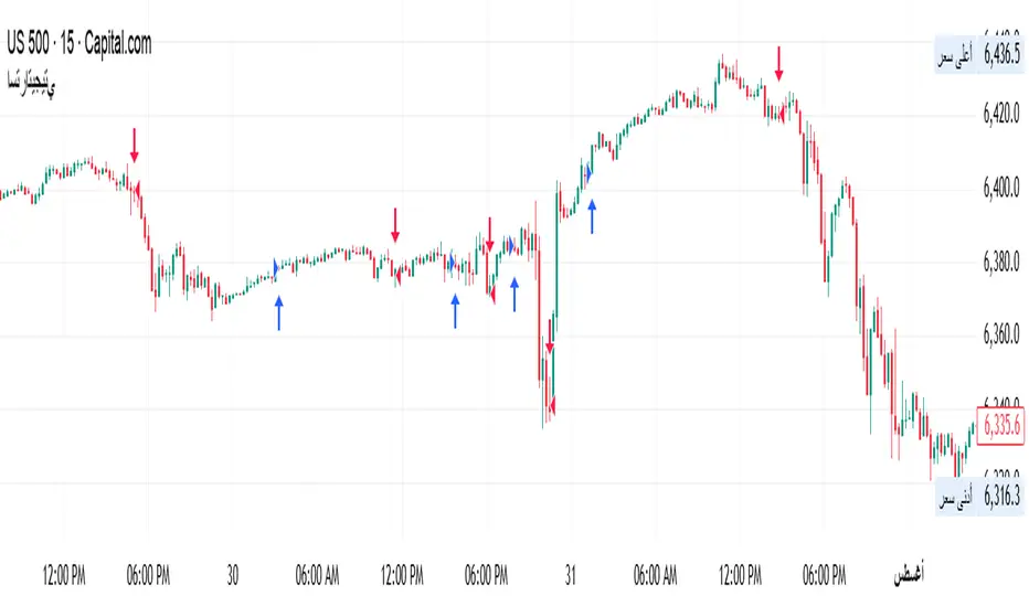
SP500 Session Gap Fade StrategySummary in one paragraph
SPX Session Gap Fade is an intraday gap fade strategy for index futures, designed around regular cash sessions on five minute charts. It helps you participate only when there is a full overnight or pre session gap and a valid intraday session window, instead of trading every open. The original part is the gap distance engine which anchors both stop and optional target to the previous session reference close at a configurable flat time, so every trade’s risk scales with the actual gap size rather than a fixed tick stop.
Scope and intent
• Markets. Primarily index futures such as ES, NQ, YM, and liquid index CFDs that exhibit overnight gaps and regular cash hours.
• Timeframes. Intraday timeframes from one minute to fifteen minutes. Default usage is five minute bars.
• Default demo used in the publication. Symbol CME:ES1! on a five minute chart.
• Purpose. Provide a simple, transparent way to trade opening gaps with a session anchored risk model and forced flat exit so you are not holding into the last part of the session.
• Limits. This is a strategy. Orders are simulated on standard candles only.
Originality and usefulness
• Unique concept or fusion. The core novelty is the combination of a strict “full gap” entry condition with a session anchored reference close and a gap distance based TP and SL engine. The stop and optional target are symmetric multiples of the actual gap distance from the previous session’s flat close, rather than fixed ticks.
• Failure mode it addresses. Fixed sized stops do not scale when gaps are unusually small or unusually large, which can either under risk or over risk the account. The session flat logic also reduces the chance of holding residual positions into late session liquidity and news.
• Testability. All key pieces are explicit in the Inputs: session window, minutes before session end, whether to use gap exits, whether TP or SL are active, and whether to allow candle based closes and forced flat. You can toggle each component and see how it changes entries and exits.
• Portable yardstick. The main unit is the absolute price gap between the entry bar open and the previous session reference close. tp_mult and sl_mult are multiples of that gap, which makes the risk model portable across contracts and volatility regimes.
Method overview in plain language
The strategy first defines a trading session using exchange time, for example 08:30 to 15:30 for ES day hours. It also defines a “flat” time a fixed number of minutes before session end. At the flat bar, any open position is closed and the bar’s close price is stored as the reference close for the next session. Inside the session, the strategy looks for a full gap bar relative to the prior bar: a gap down where today’s high is below yesterday’s low, or a gap up where today’s low is above yesterday’s high. A full gap down generates a long entry; a full gap up generates a short entry. If the gap risk engine is enabled and a valid reference close exists, the strategy measures the distance between the entry bar open and that reference close. It then sets a stop and optional target as configurable multiples of that gap distance and manages them with strategy.exit. Additional exits can be triggered by a candle color flip or by the forced flat time.
Base measures
• Range basis. The main unit is the absolute difference between the current entry bar open and the stored reference close from the previous session flat bar. That value is used as a “gap unit” and scaled by tp_mult and sl_mult to build the target and stop.
Components
• Component one: Gap Direction. Detects full gap up or full gap down by comparing the current high and low to the previous bar’s high and low. Gap down signals a long fade, gap up signals a short fade. There is no smoothing; it is a strict structural condition.
• Component two: Session Window. Only allows entries when the current time is within the configured session window. It also defines a flat time before the session end where positions are forced flat and the reference close is updated.
• Component three: Gap Distance Risk Engine. Computes the absolute distance between the entry open and the stored reference close. The stop and optional target are placed as entry ± gap_distance × multiplier so that risk scales with gap size.
• Optional component: Candle Exit. If enabled, a bullish bar closes short positions and a bearish bar closes long positions, which can shorten holding time when price reverses quickly inside the session.
• Session windows. Session logic uses the exchange time of the chart symbol. When changing symbols or venues, verify that the session time string still matches the new instrument’s cash hours.
Fusion rule
All gates are hard conditions rather than weighted scores. A trade can only open if the session window is active and the full gap condition is true. The gap distance engine only activates if a valid reference close exists and use_gap_risk is on. TP and SL are controlled by separate booleans so you can use SL only, TP only, or both. Long and short are symmetric by construction: long trades fade full gap downs, short trades fade full gap ups with mirrored TP and SL logic.
Signal rule
• Long entry. Inside the active session, when the current bar shows a full gap down relative to the previous bar (current high below prior low), the strategy opens a long position. If the gap risk engine is active, it places a gap based stop below the entry and an optional target above it.
• Short entry. Inside the active session, when the current bar shows a full gap up relative to the previous bar (current low above prior high), the strategy opens a short position. If the gap risk engine is active, it places a gap based stop above the entry and an optional target below it.
• Forced flat. At the configured flat time before session end, any open position is closed and the close price of that bar becomes the new reference close for the following session.
• Candle based exit. If enabled, a bearish bar closes longs, and a bullish bar closes shorts, regardless of where TP or SL sit, as long as a position is open.
What you will see on the chart
• Markers on entry bars. Standard strategy entry markers labeled “long” and “short” on the gap bars where trades open.
• Exit markers. Standard exit markers on bars where either the gap stop or target are hit, or where a candle exit or forced flat close occurs. Exit IDs “long_gap” and “short_gap” label gap based exits.
• Reference levels. Horizontal lines for the current long TP, long SL, short TP, and short SL while a position is open and the gap engine is enabled. They update when a new trade opens and disappear when flat.
• Session background. This version does not add background shading for the session; session logic runs internally based on time.
• No on chart table. All decisions are visible through orders and exit levels. Use the Strategy Tester for performance metrics.
Inputs with guidance
Session Settings
• Trading session (sess). Session window in exchange time. Typical value uses the regular cash session for each contract, for example “0830-1530” for ES. Adjust if your broker or symbol uses different hours.
• Minutes before session end to force exit (flat_before_min). Minutes before the session end where positions are forced flat and the reference close is stored. Typical range is 15 to 120. Raising it closes trades earlier in the day; lowering it allows trades later in the session.
Gap Risk
• Enable gap based TP/SL (use_gap_risk). Master switch for the gap distance exit engine. Turning it off keeps entries and forced flat logic but removes automatic TP and SL placement.
• Use TP limit from gap (use_gap_tp). Enables gap based profit targets. Typical values are true for structured exits or false if you want to manage exits manually and only keep a stop.
• Use SL stop from gap (use_gap_sl). Enables gap based stop losses. This should normally remain true so that each trade has a defined initial risk in ticks.
• TP multiplier of gap distance (tp_mult). Multiplier applied to the gap distance for the target. Typical range is 0.5 to 2.0. Raising it places the target further away and reduces hit frequency.
• SL multiplier of gap distance (sl_mult). Multiplier applied to the gap distance for the stop. Typical range is 0.5 to 2.0. Raising it widens the stop and increases risk per trade; lowering it tightens the stop and may increase the number of small losses.
Exit Controls
• Exit with candle logic (use_candle_exit). If true, closes shorts on bullish candles and longs on bearish candles. Useful when you want to react to intraday reversal bars even if TP or SL have not been reached.
• Force flat before session end (use_forced_flat). If true, guarantees you are flat by the configured flat time and updates the reference close. Turn this off only if you understand the impact on overnight risk.
Filters
There is no separate trend or volatility filter in this version. All trades depend on the presence of a full gap bar inside the session. If you need extra filtering such as ATR, volume, or higher timeframe bias, they should be added explicitly and documented in your own fork.
Usage recipes
Intraday conservative gap fade
• Timeframe. Five minute chart on ES regular session.
• Gap risk. use_gap_risk = true, use_gap_tp = true, use_gap_sl = true.
• Multipliers. tp_mult around 0.7 to 1.0 and sl_mult around 1.0.
• Exits. use_candle_exit = false, use_forced_flat = true. Focus on the structured TP and SL around the gap.
Intraday aggressive gap fade
• Timeframe. Five minute chart.
• Gap risk. use_gap_risk = true, use_gap_tp = false, use_gap_sl = true.
• Multipliers. sl_mult around 0.7 to 1.0.
• Exits. use_candle_exit = true, use_forced_flat = true. Entries fade full gaps, stops are tight, and candle color flips flatten trades early.
Higher timeframe gap tests
• Timeframe. Fifteen minute or sixty minute charts on instruments with regular gaps.
• Gap risk. Keep use_gap_risk = true. Consider slightly higher sl_mult if gaps are structurally wider on the higher timeframe.
• Note. Expect fewer trades and be careful with sample size; multi year data is recommended.
Properties visible in this publication
• On average our risk for each position over the last 200 trades is 0.4% with a max intraday loss of 1.5% of the total equity in this case of 100k $ with 1 contract ES. For other assets, recalculations and customizations has to be applied.
• Initial capital. 100 000.
• Base currency. USD.
• Default order size method. Fixed with size 1 contract.
• Pyramiding. 0.
• Commission. Flat 2 USD per order in the Strategy Tester Properties. (2$ buying + 2$selling)
• Slippage. One tick in the Strategy Tester Properties.
• Process orders on close. ON.
Realism and responsible publication
• No performance claims are made. Past results do not guarantee future outcomes.
• Costs use a realistic flat commission and one tick of slippage per trade for ES class futures.
• Default sizing with one contract on a 100 000 reference account targets modest per trade risk. In practice, extreme slippage or gap through events can exceed this, so treat the one and a half percent risk target as a design goal, not a guarantee.
• All orders are simulated on standard candles. Shapes can move while a bar is forming and settle on bar close.
Honest limitations and failure modes
• Economic releases, thin liquidity, and limit conditions can break the assumptions behind the simple gap model and lead to slippage or skipped fills.
• Symbols with very frequent or very large gaps may require adjusted multipliers or alternative risk handling, especially in high volatility regimes.
• Very quiet periods without clean gaps will produce few or no trades. This is expected behavior, not a bug.
• Session windows follow the exchange time of the chart. Always confirm that the configured session matches the symbol.
• When both the stop and target lie inside the same bar’s range, the TradingView engine decides which is hit first based on its internal intrabar assumptions. Without bar magnifier, tie handling is approximate.
Legal
Education and research only. This strategy is not investment advice. You remain responsible for all trading decisions. Always test on historical data and in simulation with realistic costs before considering any live use.

XAU/USD Weekly Volatility Strategy by WeTradeAIWeTradeAI - XAU/USD Weekly Volatility Strategy
This strategy is designed for Gold (XAU/USD) trading, leveraging a weekly market structure and volatility projection model. It dynamically identifies high-probability zones based on the prior week’s price action and adapts to intraday movement.
🔍 Core Logic:
Weekly High, Low & Midpoint: Defines structural balance for directional bias.
Projected Volatility Zones:
Green Zone: Upward projection from last week’s low.
Red Zone: Downward projection from last week’s high.
Half-Volatility Lines: Act as breakout or reversal triggers.
Monday Open: Serves as a temporary directional reference until midweek.
Daily High, Low, and Mid: Used for intraday stop-loss placement and validation.
🎯 Trade Entries:
Breakout Entries: Triggered when price breaks and holds above/below the Half-Vol levels.
Reversal Entries: Triggered by strong rejections near outer zones, reverting back toward equilibrium.
🛡️ Risk Management:
Dynamic Stop-Loss: Based on the previous day’s midpoint.
⏱️ Multi-Timeframe Usage:
4H – Weekly structure & context
1H – Trend alignment
15M – Precision entries

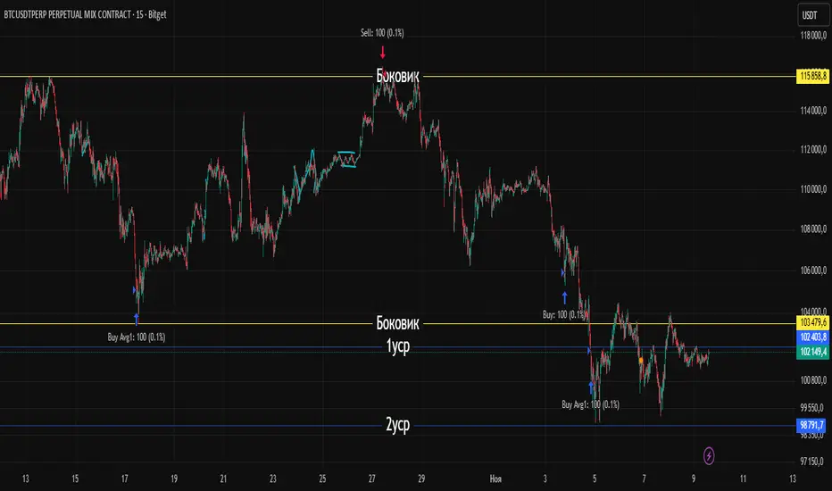
KriptoBotik 5 min TFCryptobot is effective on a 5-minute timeframe on any coin (with appropriate settings), with a grid of 10 averages, where each average is equal to the sum of previous entries, with a stop-loss. It can be configured for both local volatility and strong channel coverage, with adjustable entry amounts for each average and a percentage grid between averages. It can be connected to any exchange via API keys.

KriptoBotik 15 min TFCryptobot is effective on a 15-minute timeframe on any coin (with appropriate settings), with a grid of 10 averages (5 averages are sufficient with global settings), where each average is equal to the sum of previous entries, with a stop-loss. It can be configured for both local volatility and strong channel coverage, with adjustable entry amounts for each average and a percentage grid between averages. It can be connected to any exchange using API keys.
Bybit BTCUSD.P 자동매매 전략 v12 (Pi Cycle 비율 필터)Abstract
Sigma Trinity Model is an educational framework that studies how three layers of market behavior interact within the same trend: (1) structural momentum (Rasta), (2) internal strength (RSI), and (3) continuation/compounding structure (Pyramid). The model deliberately combines bar-close momentum logic with intrabar, wick-aware strength checks to help users see how reversals form, confirm, and extend. It is not a signal service or automation tool; it is a transparent learning instrument for chart study and backtesting.
Why this is not “just a mashup”
Many scripts merge indicators without explaining the purpose. Sigma Trinity is a coordinated, three-engine study designed for a specific learning goal:
Rasta (structure): defines when momentum actually flips using a dual-line EMA vs smoothed EMA. It gives the entry/exit framework on bar close for clean historical study.
RSI (energy): measures internal strength with wick-aware triggers. It uses RSI of LOW (for bottom touches/reclaims) and RSI of HIGH (for top touches/exhaustion) so users can see intrabar strength/weakness that the close can hide.
Pyramid (progression): demonstrates how continuation behaves once momentum and strength align. It shows the logic of adds (compounding) as a didactic layer, also on bar close to keep historical alignment consistent.
These three roles are complementary, not redundant: structure → strength → progression.
Architecture Overview
Execution model
Rasta & Pyramid: bar close only by default (historically stable, easy to audit).
RSI: per tick (realtime) with bar-close backup by default, using RSI of LOW for entries and RSI of HIGH for exits. This makes the module sensitive to intra-bar wicks while still giving a close-based safety net for backtests.
Stops (optional in strategy builds): wick-accurate: trail arms/ratchets on HIGH; stop hit checks with LOW (or Close if selected) with a small undershoot buffer to avoid micro-noise hits.
Visual model
Dual lines (EMA vs smoothed EMA) for Rasta + color fog to see direction and compression/expansion.

PDHL Breakout SMA50 By Ajit TiwariThis indicator help you to find buy sell from previous day high low basis

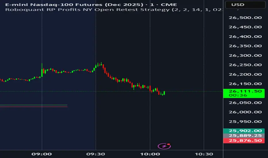
Roboquant RP Profits NY Open Retest StrategyRoboquant RP Profits NY Open Retest Strategy A good strategy for CL
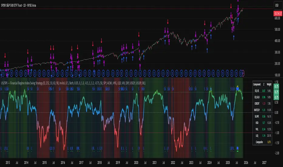
US/SPY- Financial Regime Index Swing Strategy Credits: concept inspired by EdgeTools Bloomberg Financial Conditions Index (Proxy)
Improvements: eight component basket, inverse volatility weights, winsorization option( statistical technique used to limit the influence of outliers in a dataset by replacing extreme values with less extreme ones, rather than removing them entirely), slope and price gates, exit guards, table and gradients.
Summary in one paragraph
A macro regime swing strategy for index ETFs, futures, FX majors, and large cap equities on daily calculation with optional lower time execution. It acts only when a composite Financial Conditions proxy plus slope and an optional price filter align. Originality comes from an eight component macro basket with inverse volatility weights and winsorized return z scores that produce a portable yardstick.
Scope and intent
Markets: SPY and peers, ES futures, ACWI, liquid FX majors, BTC, large cap equities.
Timeframes: calculation daily by default, trade on any chart.
Default demo: SPY on Daily.
Purpose: convert broad financial conditions into clear swing bias and exits.
Originality and usefulness
Unique fusion: return z scores for eight liquid proxies with inverse volatility weighting and optional winsorization, then slope and price gates.
Failure mode addressed: false starts in chop and early shorts during easy liquidity.
Testability: all knobs are inputs and the table shows components and weights.
Portable yardstick: z scores center at zero so thresholds transfer across symbols.
Method overview in plain language
Base measures
Return basis: natural log return over a configurable window, standardized to a z score. Winsorization optional to cap extremes.
Components
EQ US and EQ GLB measure equity tone.
CREDIT uses LQD over HYG. Higher credit quality outperformance is risk off so sign is flipped after z score.
RATES2Y uses two year yield, sign flipped.
SLOPE uses ten minus two year yield spread.
USD uses DXY, sign flipped.
VOL uses VIX, sign flipped.
LIQ uses BIL over SPY, sign flipped.
Each component is smoothed by the composite EMA.
Fusion rule
Weighted sum where weights are equal or inverse volatility with exponent gamma, normalized to percent so they sum to one.
Signal rule
Long when composite crosses up the long threshold and its slope is positive and price is above the SMA filter, or when composite is above the configured always long floor.
Short when composite crosses down the short threshold and its slope is negative and price is below the SMA filter.
Long exit on cross down of the long exit line or on a fresh short signal.
Short exit on cross up of the short exit line or on a fresh long signal, or when composite falls below the force short exit guard.
What you will see on the chart
Markers on suggestion bars: L for long, S for short, LX and SX for exits.
Reference lines at zero and soft regime bands at plus one and minus one.
Optional background gradient by regime intensity.
Compact table with component z, weight percent, and composite readout.
Table fields and quick reading guide
Component: EQ US, EQ GLB, CREDIT, RATES2Y, SLOPE, USD, VOL, LIQ.
Z: current standardized value, green for positive risk tone where applicable.
Weight: contribution percent after normalization.
Composite: current index value.
Reading tip: a broadly green Z column with slope positive often precedes better long context.
Inputs with guidance
Setup
Calc timeframe: default Daily. Leave blank to inherit chart.
Lookback: 50 to 1500. Larger length stabilizes regimes and delays turns.
EMA smoothing: 1 to 200. Higher smooths noise and delays signals.
Normalization
Winsorize z at ±3: caps extremes to reduce one off shocks.
Return window for equities: 5 to 260. Shorter reacts faster.
Weighting
Weight lookback: 20 to 520.
Weight mode: Equal or InvVol.
InvVol exponent gamma: 0.1 to 3. Higher compresses noisy components more.
Signals
Trade side: Long Short or Both.
Entry threshold long and short: portable z thresholds.
Exit line long and short: soft exits that give back less.
Slope lookback bars: 1 to 20.
Always long floor bfci ≥ X: macro easy mode keep long.
Force short exit when bfci < Y: macro stress guard.
Confirm
Use price trend filter and Price SMA length.
View
Glow line and Show component table.
Symbols
SPY ACWI HYG LQD VIX DXY US02Y US10Y BIL are defaults and can be changed.
Realism and responsible publication
No performance claims. Past is not future.
Shapes can move intrabar and settle on close.
Execution is on standard candles only.
Honest limitations and failure modes
Major economic releases and illiquid sessions can break assumptions.
Very quiet regimes reduce contrast. Use longer windows or higher thresholds.
Component proxies are ETFs and indexes and cannot match a proprietary FCI exactly.
Strategy notice
Orders are simulated on standard candles. All security calls use lookahead off. Nonstandard chart types are not supported for strategies.
Entries and exits
Long rule: bfci cross above long threshold with positive slope and optional price filter OR bfci above the always long floor.
Short rule: bfci cross below short threshold with negative slope and optional price filter.
Exit rules: long exit on bfci cross below long exit or on a short signal. Short exit on bfci cross above short exit or on a long signal or on force close guard.
Position sizing
Percent of equity by default. Keep target risk per trade low. One percent is a sensible starting point. For this example we used 3% of the total capital
Commisions
We used a 0.05% comission and 5 tick slippage
Legal
Education and research only. Not investment advice. Test in simulation first. Use realistic costs.
Confluence Dashboard + Strategy [Daily + Weekly Adaptive]Removed duplicate strategy() declarations
Scoped getWeeklyBias() safely with correct request.security() usage
Ensured all variables are declared before use
Aligned background shading with bias logic
Streamlined signal tier logic to avoid overlap
Integrated strategy entries/exits cleanly

DCA with the Money Supply Index DCA with the Money Supply Index (MSI) by zdmre
This strategy is based on the Money Supply Index (MSI) by zdmre and enhances it with two functional options for users: a DCA (Dollar-Cost Averaging) approach and a signal-based buy/sell mode. It’s designed to help traders and investors make data-driven, disciplined entry decisions based on monetary supply trends.
🧠 Concept Overview
The Money Supply Index (MSI) provides insight into how liquidity (money supply) influences market movements. This strategy builds upon that foundation by allowing users to either:
Accumulate positions over time using DCA, based on favorable MSI conditions.
Execute a single buy and sell trade, optimized for bull market conditions.
⚙️ Inputs Explained
General Parameters
Start Bar Index / Stop Bar Index
Defines the range of bars (historical data) for backtesting or strategy visualization.
Long DCA
Activates the DCA mode. If unchecked, the strategy operates in single-entry/single-exit signal mode.
Trading Signal
Enables signal-based entries and exits when the MSI reaches predefined thresholds.
DCA Parameters
Entry Value
The MSI value that triggers a DCA buy event. When the MSI crosses below this value, the strategy considers it a favorable moment to deploy the saved capital.
Saved Amount
The amount of money set aside regularly (e.g., monthly) for investment. This simulates the DCA effect by accumulating capital and deploying it when conditions are optimal.
Data Inputs
Money Supply
The data source for the Money Supply Index (default: ECONOMICS:USM2).
Relational Symbol
The market instrument to compare against the money supply (default: NASDAQ_DLY:NDX). This allows the strategy to measure liquidity impact on a specific market.
Chart Display Options
You can toggle these metrics on the chart for better visualization:
Entry Price (green) – The price level of executed buys.
Cash Balance (yellow) – Remaining uninvested capital.
Invested Capital (red) – Total amount currently invested.
Current Value (blue) – The current valuation of the investment.
Profit (purple) – The total realized and unrealized profit.
Trades on Chart / Signal Labels / Quantity – Enables trade markers, signal text, and position size visualization.
📈 How the Strategy Works
1️⃣ DCA Mode
In DCA mode, the strategy simulates periodic savings and only invests when the MSI indicates favorable liquidity conditions (based on the Entry Value).
This approach aims to achieve the best possible average entry price over time — a powerful strategy for long-term investors seeking stable accumulation with reduced emotional bias.
2️⃣ Signal-Based Mode
In signal mode (with DCA disabled), the strategy performs one buy and one sell trade based on MSI turning points.
It’s most effective during bull markets, where liquidity expansion supports upward momentum.
This mode helps identify high-probability entry and exit zones rather than averaging in continuously.
💡 Additional Notes
This strategy includes helpful metrics to monitor your personal investment performance — showing invested capital, cash reserves, and profit in real-time.
The goal is to combine macroeconomic insight (money supply) with disciplined execution and capital management.
⚠️ Disclaimer
This strategy is for educational and research purposes only. It does not constitute financial advice. Always conduct your own analysis before making investment decisions.

Order Block Volumatic FVG StrategyInspired by: Volumatic Fair Value Gaps —
License: CC BY-NC-SA 4.0 (Creative Commons Attribution–NonCommercial–ShareAlike).
This script is a non-commercial derivative work that credits the original author and keeps the same license.
What this strategy does
This turns BigBeluga’s visual FVG concept into an entry/exit strategy. It scans bullish and bearish FVG boxes, measures how deep price has mitigated into a box (as a percentage), and opens a long/short when your mitigation threshold and filters are satisfied. Risk is managed with a fixed Stop Loss % and a Trailing Stop that activates only after a user-defined profit trigger.
Additions vs. the original indicator
✅ Strategy entries based on % mitigation into FVGs (long/short).
✅ Lower-TF volume split using upticks/downticks; fallback if LTF data is missing (distributes prior bar volume by close’s position in its H–L range) to avoid NaN/0.
✅ Per-FVG total volume filter (min/max) so you can skip weak boxes.
✅ Age filter (min bars since the FVG was created) to avoid fresh/immature boxes.
✅ Bull% / Bear% share filter (the 46%/53% numbers you see inside each FVG).
✅ Optional candle confirmation and cooldown between trades.
✅ Risk management: fixed SL % + Trailing Stop with a profit trigger (doesn’t trail until your trigger is reached).
✅ Pine v6 safety: no unsupported args, no indexof/clamp/when, reverse-index deletes, guards against zero/NaN.
How a trade is decided (logic overview)
Detect FVGs (same rules as the original visual logic).
For each FVG currently intersected by the bar, compute:
Mitigation % (how deep price has entered the box).
Bull%/Bear% split (internal volume share).
Total volume (printed on the box) from LTF aggregation or fallback.
Age (bars) since the box was created.
Apply your filters:
Mitigation ≥ Long/Short threshold.
Volume between your min and max (if enabled).
Age ≥ min bars (if enabled).
Bull% / Bear% within your limits (if enabled).
(Optional) the current candle must be in trade direction (confirm).
If multiple FVGs qualify on the same bar, the strategy uses the most recent one.
Enter long/short (no pyramiding).
Exit with:
Fixed Stop Loss %, and
Trailing Stop that only starts after price reaches your profit trigger %.
Input settings (quick guide)
Mitigation source: close or high/low. Use high/low for intrabar touches; close is stricter.
Mitigation % thresholds: minimal mitigation for Long and Short.
TOTAL Volume filter: skip FVGs with too little/too much total volume (per box).
Bull/Bear share filter: require, e.g., Long only if Bull% ≥ 50; avoid Short when Bull% is high (Short Bull% max).
Age filter (bars): e.g., ≥ 20–30 bars to avoid fresh boxes.
Confirm candle: require candle direction to match the trade.
Cooldown (bars): minimum bars between entries.
Risk:
Stop Loss % (fixed from entry price).
Activate trailing at +% profit (the trigger).
Trailing distance % (the trailing gap once active).
Lower-TF aggregation:
Auto: TF/Divisor → picks 1/3/5m automatically.
Fixed: choose 1/3/5/15m explicitly.
If LTF can’t be fetched, fallback allocates prior bar’s volume by its close position in the bar’s H–L.
Suggested starting presets (you should optimize per market)
Mitigation: 60–80% for both Long/Short.
Bull/Bear share:
Long: Bull% ≥ 50–70, Bear% ≤ 100.
Short: Bull% ≤ 60 (avoid shorting into strong support), Bear% ≥ 0–70 as you prefer.
Age: ≥ 20–30 bars.
Volume: pick a min that filters noise for your symbol/timeframe.
Risk: SL 4–6%, trailing trigger 1–2%, distance 1–2% (crypto example).
Set slippage/fees in Strategy Properties.
Notes, limitations & best practices
Data differences: The LTF split uses request.security_lower_tf. If the exchange/data feed has sparse LTF data, the fallback kicks in (it’s deliberate to avoid NaNs but is a heuristic).
Real-time vs backtest: The current bar can update until close; results on historical bars use closed data. Use “Bar Replay” to understand intrabar effects.
No pyramiding: Only one position at a time. Modify pyramiding in the header if you need scaling.
Assets: For spot/crypto, TradingView “volume” is exchange volume; in some markets it may be tick volume—interpret filters accordingly.
Risk disclosure: Past performance ≠ future results. Use appropriate position sizing and risk controls; this is not financial advice.
Credits
Visual FVG concept and original implementation: BigBeluga.
This derivative strategy adds entry/exit logic, volume/age/share filters, robust LTF handling, and risk management while preserving the original spirit.
License remains CC BY-NC-SA 4.0 (non-commercial, attribution required, share-alike).