Multi Brownian Forecast📊 Multi Brownian Forecast (Time-Adaptive, Probabilistic)
This indicator uses a sophisticated Geometric Brownian Motion (GBM) Monte Carlo simulation to project future price paths. It adapts to any chart timeframe and provides quantitative, multi-period probability signals.
---
🧠 Core Mathematical Methodology
The model relies on GBM, which is a continuous-time stochastic process that models asset prices.
1. Historical Analysis (Drift & Volatility):
* The script first calculates Logarithmic Returns over a user-defined Historical Lookback (Hours) .
* Drift ($\mu$): Computed as the average of the log returns.
* Volatility ($\sigma$): Computed as the standard deviation of the log returns.
* These values are then time-adapted to an hourly step, compensating for the chart's current timeframe (e.g., 5-minute, 1-hour).
2. Monte Carlo Simulation:
* It runs a specified Number of Simulations (e.g., 1000).
* For each simulation, the price is stepped forward hourly using the GBM formula, which incorporates the calculated drift and a random shock drawn from a normal distribution (generated via the Box-Muller transform ).
---
✨ Key Features
Probabilistic Quartile Forecast: Plots a dynamic "cone" of probability on the chart. It shows key price percentiles (Q1, Q2/Median, Q3, and Q4/Outer Bound) at the forecast's expiration, visualizing the expected range of price outcomes based on the simulations.
Multi-Period Probability Signals: This is the core signal feature. Users can define multiple, independent forecast periods (e.g., 4h, 16h, 48h) in a comma-separated list.
* For each period, a Probability Up and Probability Down is calculated based on hitting a custom Target Price Change (%) (e.g., 2%) at a certain confidence level given a simulation over the historical backlook.
* The probabilities are displayed in a chart table. The cell text turns white if the calculated probability exceeds the user-defined Signal Confidence (%) .
Conditional Fibonacci Retracement: Optionally displays a Fibonacci Retracement on the chart. This feature is only activated when one of the multi-period signals reaches its minimum confidence threshold, providing a contextual technical level when a probabilistic edge is found.
Brownian

Brownian Motion Probabilistic Forecasting (Time Adaptive)Probabilistic Price Forecast Indicator
Overview
The Probabilistic Price Forecast is an advanced technical analysis tool designed for the TradingView platform. Instead of predicting a single future price, this indicator uses a Monte Carlo simulation to model thousands of potential future price paths, generating a cone of possibilities and calculating the probability of specific outcomes.
This allows traders to move beyond simple price targets and ask more sophisticated questions, such as: "What is the probability that this stock will increase by 5% over the next 24 hours?"
Core Concept: Geometric Brownian Motion
The indicator's forecasting model is built on the principles of Geometric Brownian Motion (GBM) , a widely accepted mathematical model for describing the random movements of financial asset prices. The core idea is that the next price step is a function of the asset's historical trend (drift), its volatility, and a random "shock."
The formula used to project each price step in the simulation is:
next_price = current_price * exp( (μ - (σ²/2))Δt + σZ√(Δt) )
Where:
μ (mu) represents the drift , which is the average historical return.
σ (sigma) represents the volatility , measured by the standard deviation of historical returns.
Z is a random variable from a standard normal distribution, representing the random "shock" or new information affecting the price.
Δt (delta t) is the time step for each projection.
How It Works
The indicator performs a comprehensive analysis on the most recent bar of the chart:
**Historical Analysis**: It first analyzes a user-defined historical period (e.g., the last 240 hours of price data) to calculate the asset's historical drift (μ) and volatility (σ) from its logarithmic returns.
**Monte Carlo Simulation**: It then runs thousands of simulations (e.g., 2000) of future price paths over a specified forecast period (e.g., the next 24 hours). Each path is unique due to the random shock (Z) applied at every step.
**Probability Distribution**: After all simulations are complete, it collects the final price of each path and sorts them to build a probability distribution of potential outcomes.
**Visualization and Signaling**: Finally, it visualizes this distribution on the chart and generates signals based on the user's criteria.
Key Features & Configuration
The indicator is highly configurable, allowing you to tailor its analysis to your specific needs.
Time-Adaptive Periods
The lookback and forecast periods are defined in hours , not bars. The script automatically converts these hour-based inputs into the correct number of bars based on the chart's current timeframe, ensuring the analysis remains consistent across different chart resolutions.
Forecast Quartiles
You can visualize the forecast as a "cone of probability" on the chart. The indicator draws lines and a shaded area representing the price levels for different quartiles (percentiles) of the simulation results. By default, this shows the range between the 25th and 95th percentiles.
Independent Bullish and Bearish Signals
The indicator allows you to set independent criteria for bullish and bearish signals, providing greater flexibility. You can configure:
A bullish signal for an X% confidence of a Y% price increase.
A bearish signal for a W% confidence of a Z% price decrease.
For example, you can set it to alert you for a 90% chance of a 2% drop, while simultaneously looking for a 60% chance of a 10% rally.
How to Interpret the Indicator
The Forecast Cone : The blue shaded area on the chart represents the probable range of future prices. The width of the cone indicates the expected volatility; a wider cone means higher uncertainty. The price labels on the right side of the cone show the calculated percentile levels at the end of the forecast period.
Green Signal Label : A green "UP signal" label appears when the probability of the price increasing by your target percentage exceeds your defined confidence level.
Red Signal Label : A red "DOWN signal" label appears when the probability of the price decreasing by your target percentage exceeds your confidence level.
This tool provides a statistical edge for understanding future possibilities but should be used in conjunction with other analysis techniques.

Garman-Klass-Yang-Zhang Historical Volatility Bands [Loxx]Garman-Klass-Yang-Zhang Historical Volatility Bands are constructed using:
Average as the middle line.
Upper and lower bands using the Garman-Klass-Yang-Zhang Historical Volatility Bands for bands calculation.
What is Garman-Klass-Yang-Zhang Historical Volatility?
Yang and Zhang derived an extension to the Garman Klass historical volatility estimator that allows for opening jumps. It assumes Brownian motion with zero drift. This is currently the preferred version of open-high-low-close volatility estimator for zero drift and has an efficiency of 8 times the classic close-to-close estimator. Note that when the drift is nonzero, but instead relative large to the volatility, this estimator will tend to overestimate the volatility. The Garman-Klass-Yang-Zhang Historical Volatility calculation is as follows:
GKYZHV = sqrt((Z/n) * sum((log(open(k)/close(k-1)))^2 + (0.5*(log(high(k)/low(k)))^2) - (2*log(2) - 1)*(log(close(k)/open(2:end)))^2))
The color of the middle line, unlike the bands colors, has 3 colors. When colors of the bands are the same, then the middle line has the same color, otherwise it's white.
Included
Alerts
Signals
Loxx's Expanded Source Types
Bar coloring
Related Indicators
Garman & Klass Estimator Historical Volatility Bands

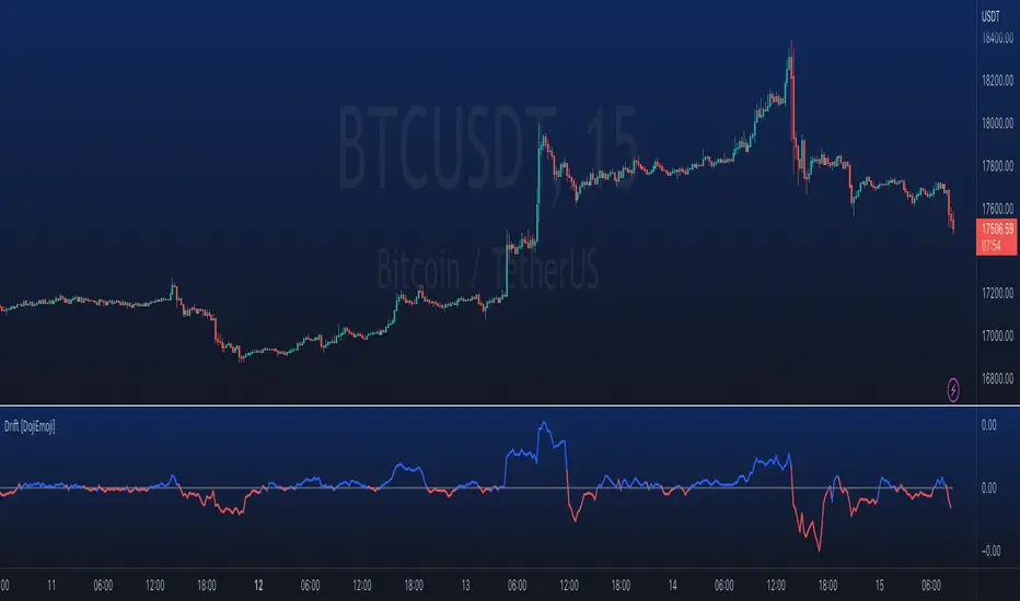
Drift Study (Inspired by Monte Carlo Simulations with BM) [KL]Inspired by the Brownian Motion ("BM") model that could be applied to conducting Monte Carlo Simulations, this indicator plots out the Drift factor contributing to BM.
Interpretation : If the Drift value is positive, then prices are possibly moving in an uptrend. Vice versa for negative drifts.
Hurst ExponentThis is an aproximation on Tradingview of the Hurst Exponent.
Its quite computational expensive, so it has been simplify and sample size reduced.
If any has an idea on how to create the real Hurst Exponent here, Ill be happy to hear and help.
