FunctionBaumWelch
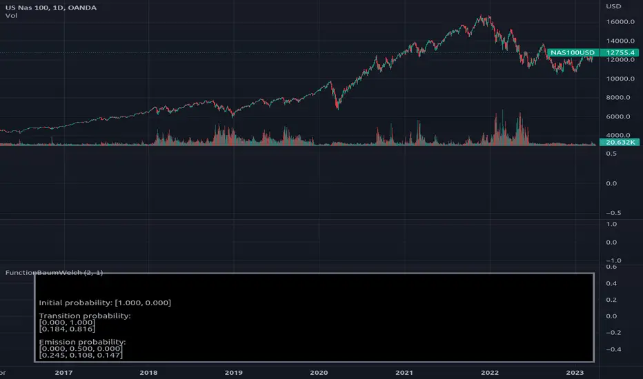
Baum-Welch Algorithm, also known as Forward-Backward Algorithm, uses the well known EM algorithm
to find the maximum likelihood estimate of the parameters of a hidden Markov model given a set of observed
feature vectors.
---
### Function List:
> `forward (array<float> pi, matrix<float> a, matrix<float> b, array<int> obs)`
> `forward (array<float> pi, matrix<float> a, matrix<float> b, array<int> obs, bool scaling)`
> `backward (matrix<float> a, matrix<float> b, array<int> obs)`
> `backward (matrix<float> a, matrix<float> b, array<int> obs, array<float> c)`
> `baumwelch (array<int> observations, int nstates)`
> `baumwelch (array<int> observations, array<float> pi, matrix<float> a, matrix<float> b)`
---
### Reference:
> en.wikipedia.org/wiki/Baum–Welch_algorithm
> github.com/alexsosn/MarslandMLAlgo/blob/4277b24db88c4cb70d6b249921c5d21bc8f86eb4/Ch16/HMM.py
> en.wikipedia.org/wiki/Forward_algorithm
> rdocumentation.org/packages/HMM/versions/1.0.1/topics/forward
> rdocumentation.org/packages/HMM/versions/1.0.1/topics/backward
forward(pi, a, b, obs)
Computes forward probabilities for state `X` up to observation at time `k`, is defined as the
probability of observing sequence of observations `e_1 ... e_k` and that the state at time `k` is `X`.
Parameters:
pi (float[]): Initial probabilities.
a (matrix<float>): Transmissions, hidden transition matrix a or alpha = transition probability matrix of changing
states given a state matrix is size (M x M) where M is number of states.
b (matrix<float>): Emissions, matrix of observation probabilities b or beta = observation probabilities. Given
state matrix is size (M x O) where M is number of states and O is number of different
possible observations.
obs (int[]): List with actual state observation data.
Returns: - `matrix<float> _alpha`: Forward probabilities. The probabilities are given on a logarithmic scale (natural logarithm). The first
dimension refers to the state and the second dimension to time.
forward(pi, a, b, obs, scaling)
Computes forward probabilities for state `X` up to observation at time `k`, is defined as the
probability of observing sequence of observations `e_1 ... e_k` and that the state at time `k` is `X`.
Parameters:
pi (float[]): Initial probabilities.
a (matrix<float>): Transmissions, hidden transition matrix a or alpha = transition probability matrix of changing
states given a state matrix is size (M x M) where M is number of states.
b (matrix<float>): Emissions, matrix of observation probabilities b or beta = observation probabilities. Given
state matrix is size (M x O) where M is number of states and O is number of different
possible observations.
obs (int[]): List with actual state observation data.
scaling (bool): Normalize `alpha` scale.
Returns: - #### Tuple with:
> - `matrix<float> _alpha`: Forward probabilities. The probabilities are given on a logarithmic scale (natural logarithm). The first
dimension refers to the state and the second dimension to time.
> - `array<float> _c`: Array with normalization scale.
backward(a, b, obs)
Computes backward probabilities for state `X` and observation at time `k`, is defined as the probability of observing the sequence of observations `e_k+1, ... , e_n` under the condition that the state at time `k` is `X`.
Parameters:
a (matrix<float>): Transmissions, hidden transition matrix a or alpha = transition probability matrix of changing states
given a state matrix is size (M x M) where M is number of states
b (matrix<float>): Emissions, matrix of observation probabilities b or beta = observation probabilities. given state
matrix is size (M x O) where M is number of states and O is number of different possible observations
obs (int[]): Array with actual state observation data.
Returns: - `matrix<float> _beta`: Backward probabilities. The probabilities are given on a logarithmic scale (natural logarithm). The first dimension refers to the state and the second dimension to time.
backward(a, b, obs, c)
Computes backward probabilities for state `X` and observation at time `k`, is defined as the probability of observing the sequence of observations `e_k+1, ... , e_n` under the condition that the state at time `k` is `X`.
Parameters:
a (matrix<float>): Transmissions, hidden transition matrix a or alpha = transition probability matrix of changing states
given a state matrix is size (M x M) where M is number of states
b (matrix<float>): Emissions, matrix of observation probabilities b or beta = observation probabilities. given state
matrix is size (M x O) where M is number of states and O is number of different possible observations
obs (int[]): Array with actual state observation data.
c (float[]): Array with Normalization scaling coefficients.
Returns: - `matrix<float> _beta`: Backward probabilities. The probabilities are given on a logarithmic scale (natural logarithm). The first dimension refers to the state and the second dimension to time.
baumwelch(observations, nstates)
**(Random Initialization)** Baum–Welch algorithm is a special case of the expectation–maximization algorithm used to find the
unknown parameters of a hidden Markov model (HMM). It makes use of the forward-backward algorithm
to compute the statistics for the expectation step.
Parameters:
observations (int[]): List of observed states.
nstates (int)
Returns: - #### Tuple with:
> - `array<float> _pi`: Initial probability distribution.
> - `matrix<float> _a`: Transition probability matrix.
> - `matrix<float> _b`: Emission probability matrix.
---
requires: `import RicardoSantos/WIPTensor/2 as Tensor`
baumwelch(observations, pi, a, b)
Baum–Welch algorithm is a special case of the expectation–maximization algorithm used to find the
unknown parameters of a hidden Markov model (HMM). It makes use of the forward-backward algorithm
to compute the statistics for the expectation step.
Parameters:
observations (int[]): List of observed states.
pi (float[]): Initial probaility distribution.
a (matrix<float>): Transmissions, hidden transition matrix a or alpha = transition probability matrix of changing states
given a state matrix is size (M x M) where M is number of states
b (matrix<float>): Emissions, matrix of observation probabilities b or beta = observation probabilities. given state
matrix is size (M x O) where M is number of states and O is number of different possible observations
Returns: - #### Tuple with:
> - `array<float> _pi`: Initial probability distribution.
> - `matrix<float> _a`: Transition probability matrix.
> - `matrix<float> _b`: Emission probability matrix.
---
requires: `import RicardoSantos/WIPTensor/2 as Tensor`
Biblioteca Pine
Fiel al espíritu de TradingView, el autor ha publicado este código de Pine como biblioteca de código abierto, para que otros programadores Pine de nuestra comunidad puedan reutilizarlo. ¡Enhorabuena al autor! Puede usar esta biblioteca de forma privada o en otras publicaciones de código abierto, pero la reutilización de este código en publicaciones está sujeta a nuestras Normas internas.
Exención de responsabilidad
Biblioteca Pine
Fiel al espíritu de TradingView, el autor ha publicado este código de Pine como biblioteca de código abierto, para que otros programadores Pine de nuestra comunidad puedan reutilizarlo. ¡Enhorabuena al autor! Puede usar esta biblioteca de forma privada o en otras publicaciones de código abierto, pero la reutilización de este código en publicaciones está sujeta a nuestras Normas internas.